随机算法 (Fall 2015)/Balls and Bins

Probability Space

The axiom foundation of probability theory is laid by Kolmogorov, one of the greatest mathematician of the 20th century, who advanced various very different fields of mathematics.

Definition (Probability Space)

A probability space is a triple [math]\displaystyle{ (\Omega,\Sigma,\Pr) }[/math]. [math]\displaystyle{ \Omega }[/math] is a set, called the sample space. [math]\displaystyle{ \Sigma\subseteq 2^{\Omega} }[/math] is the set of all events, satisfying: (K1). [math]\displaystyle{ \Omega\in\Sigma }[/math] and [math]\displaystyle{ \empty\in\Sigma }[/math]. (The certain event and the impossible event.) (K2). If [math]\displaystyle{ A,B\in\Sigma }[/math], then [math]\displaystyle{ A\cap B, A\cup B, A-B\in\Sigma }[/math]. (Intersection, union, and diference of two events are events). A probability measure [math]\displaystyle{ \Pr:\Sigma\rightarrow\mathbb{R} }[/math] is a function that maps each event to a nonnegative real number, satisfying (K3). [math]\displaystyle{ \Pr(\Omega)=1 }[/math]. (K4). If [math]\displaystyle{ A\cap B=\emptyset }[/math] (such events are call disjoint events), then [math]\displaystyle{ \Pr(A\cup B)=\Pr(A)+\Pr(B) }[/math]. (K5*). For a decreasing sequence of events [math]\displaystyle{ A_1\supset A_2\supset \cdots\supset A_n\supset\cdots }[/math] of events with [math]\displaystyle{ \bigcap_n A_n=\emptyset }[/math], it holds that [math]\displaystyle{ \lim_{n\rightarrow \infty}\Pr(A_n)=0 }[/math].

Remark

• In general, the set [math]\displaystyle{ \Omega }[/math] may be continuous, but we only consider discrete probability in this lecture, thus we assume that [math]\displaystyle{ \Omega }[/math] is either finite or countably infinite.
• Sometimes it is convenient to assume [math]\displaystyle{ \Sigma=2^{\Omega} }[/math], i.e. the events enumerates all subsets of [math]\displaystyle{ \Omega }[/math]. But in general, a probability space is well-defined by any [math]\displaystyle{ \Sigma }[/math] satisfying (K1) and (K2). Such [math]\displaystyle{ \Sigma }[/math] is called a [math]\displaystyle{ \sigma }[/math]-algebra defined on [math]\displaystyle{ \Omega }[/math].
• The last axiom (K5*) is redundant if [math]\displaystyle{ \Sigma }[/math] is finite, thus it is only essential when there are infinitely many events. The role of axiom (K5*) in probability theory is like Zorn's Lemma (or equivalently the Axiom of Choice) in axiomatic set theory.

Useful laws for probability can be deduced from the axioms (K1)-(K5).

Proposition

Let [math]\displaystyle{ \bar{A}=\Omega\setminus A }[/math]. It holds that [math]\displaystyle{ \Pr(\bar{A})=1-\Pr(A) }[/math]. If [math]\displaystyle{ A\subseteq B }[/math] then [math]\displaystyle{ \Pr(A)\le\Pr(B) }[/math].

Proof. The events [math]\displaystyle{ \bar{A} }[/math] and [math]\displaystyle{ A }[/math] are disjoint and [math]\displaystyle{ \bar{A}\cup A=\Omega }[/math]. Due to Axiom (K4) and (K3), [math]\displaystyle{ \Pr(\bar{A})+\Pr(A)=\Pr(\Omega)=1 }[/math]. The events [math]\displaystyle{ A }[/math] and [math]\displaystyle{ B\setminus A }[/math] are disjoint and [math]\displaystyle{ A\cup(B\setminus A)=B }[/math] since [math]\displaystyle{ A\subseteq B }[/math]. Due to Axiom (K4), [math]\displaystyle{ \Pr(A)+\Pr(B\setminus A)=\Pr(B) }[/math], thus [math]\displaystyle{ \Pr(A)\le\Pr(B) }[/math]. [math]\displaystyle{ \square }[/math]

Notation

An event [math]\displaystyle{ A\subseteq\Omega }[/math] can be represented as [math]\displaystyle{ A=\{a\in\Omega\mid \mathcal{E}(a)\} }[/math] with a predicate [math]\displaystyle{ \mathcal{E} }[/math].

The predicate notation of probability is

[math]\displaystyle{ \Pr[\mathcal{E}]=\Pr(\{a\in\Omega\mid \mathcal{E}(a)\}) }[/math].

We will mostly use the predicate notation instead of subset notation.

Conditional Probability

In probability theory, the word "condition" is a verb. "Conditioning on the event ..." means that it is assumed that the event occurs.

Definition (conditional probability)

The conditional probability that event [math]\displaystyle{ A }[/math] occurs given that event [math]\displaystyle{ B }[/math] occurs is [math]\displaystyle{ \Pr[A\mid B]=\frac{\Pr[A\wedge B]}{\Pr[B]}. }[/math]

The conditional probability is well-defined only if [math]\displaystyle{ \Pr[B]\neq0 }[/math].

For independent events [math]\displaystyle{ A }[/math] and [math]\displaystyle{ B }[/math], it holds that

[math]\displaystyle{ \Pr[A\mid B] =\Pr[A]. }[/math]

It supports our intuition that for two independent events, whether one of them occurs will not affect the chance of the other.

Law of total probability

The following fact is known as the law of total probability. It computes the probability by averaging over all possible cases.

Theorem (law of total probability)

Let [math]\displaystyle{ B_1,B_2,\ldots,B_n }[/math] be mutually disjoint events, and [math]\displaystyle{ \bigcup_{i=1}^n B_i=\Omega }[/math] is the sample space. Then for any event [math]\displaystyle{ A }[/math], [math]\displaystyle{ \Pr[A]=\sum_{i=1}^n\Pr[A\wedge B_i]=\sum_{i=1}^n\Pr[A\mid B_i]\cdot\Pr[B_i]. }[/math]

Proof. Since [math]\displaystyle{ B_1,B_2,\ldots, B_n }[/math] are mutually disjoint and [math]\displaystyle{ \bigvee_{i=1}^n B_i=\Omega }[/math], events [math]\displaystyle{ A\wedge B_1, A\wedge B_2,\ldots, A\wedge B_n }[/math] are also mutually disjoint, and [math]\displaystyle{ A=\bigcup_{i=1}^n\left(A\cap B_i\right) }[/math]. Then the additivity of disjoint events, we have [math]\displaystyle{ \Pr[A]=\sum_{i=1}^n\Pr[A\wedge B_i]=\sum_{i=1}^n\Pr[A\mid B_i]\cdot\Pr[B_i]. }[/math] [math]\displaystyle{ \square }[/math]

The law of total probability provides us a standard tool for breaking a probability into sub-cases. Sometimes this will help the analysis.

The chain rule

By the definition of conditional probability, [math]\displaystyle{ \Pr[A\mid B]=\frac{\Pr[A\wedge B]}{\Pr[B]} }[/math]. Thus, [math]\displaystyle{ \Pr[A\wedge B] =\Pr[B]\cdot\Pr[A\mid B] }[/math]. This hints us that we can compute the probability of the AND of events by conditional probabilities. Formally, we have the following theorem:

Theorem

Let [math]\displaystyle{ A_1, A_2, \ldots, A_n }[/math] be any [math]\displaystyle{ n }[/math] events. Then [math]\displaystyle{ \begin{align} \Pr\left[\bigwedge_{i=1}^n A_i\right] &= \prod_{k=1}^n\Pr\left[A_k \mid \bigwedge_{i\lt k} A_i\right]. \end{align} }[/math]

Proof. It holds that [math]\displaystyle{ \Pr[A\wedge B] =\Pr[B]\cdot\Pr[A\mid B] }[/math]. Thus, let [math]\displaystyle{ A=A_n }[/math] and [math]\displaystyle{ B=A_1\wedge A_2\wedge\cdots\wedge A_{n-1} }[/math], then [math]\displaystyle{ \begin{align} \Pr[A_1\wedge A_2\wedge\cdots\wedge A_n] &= \Pr[A_1\wedge A_2\wedge\cdots\wedge A_{n-1}]\cdot\Pr\left[A_n\mid \bigwedge_{i\lt n}A_i\right]. \end{align} }[/math] Recursively applying this equation to [math]\displaystyle{ \Pr[A_1\wedge A_2\wedge\cdots\wedge A_{n-1}] }[/math] until there is only [math]\displaystyle{ A_1 }[/math] left, the theorem is proved. [math]\displaystyle{ \square }[/math]

Random Variable

Definition (random variable)

A random variable [math]\displaystyle{ X }[/math] on a sample space [math]\displaystyle{ \Omega }[/math] is a real-valued function [math]\displaystyle{ X:\Omega\rightarrow\mathbb{R} }[/math]. A random variable X is called a discrete random variable if its range is finite or countably infinite.

For a random variable [math]\displaystyle{ X }[/math] and a real value [math]\displaystyle{ x\in\mathbb{R} }[/math], we write "[math]\displaystyle{ X=x }[/math]" for the event [math]\displaystyle{ \{a\in\Omega\mid X(a)=x\} }[/math], and denote the probability of the event by

[math]\displaystyle{ \Pr[X=x]=\Pr(\{a\in\Omega\mid X(a)=x\}) }[/math].

The independence can also be defined for variables:

Definition (Independent variables)

Two random variables [math]\displaystyle{ X }[/math] and [math]\displaystyle{ Y }[/math] are independent if and only if [math]\displaystyle{ \Pr[(X=x)\wedge(Y=y)]=\Pr[X=x]\cdot\Pr[Y=y] }[/math] for all values [math]\displaystyle{ x }[/math] and [math]\displaystyle{ y }[/math]. Random variables [math]\displaystyle{ X_1, X_2, \ldots, X_n }[/math] are mutually independent if and only if, for any subset [math]\displaystyle{ I\subseteq\{1,2,\ldots,n\} }[/math] and any values [math]\displaystyle{ x_i }[/math], where [math]\displaystyle{ i\in I }[/math], [math]\displaystyle{ \begin{align} \Pr\left[\bigwedge_{i\in I}(X_i=x_i)\right] &= \prod_{i\in I}\Pr[X_i=x_i]. \end{align} }[/math]

Note that in probability theory, the "mutual independence" is not equivalent with "pair-wise independence", which we will learn in the future.

Linearity of Expectation

Let [math]\displaystyle{ X }[/math] be a discrete random variable. The expectation of [math]\displaystyle{ X }[/math] is defined as follows.

Definition (Expectation)

The expectation of a discrete random variable [math]\displaystyle{ X }[/math], denoted by [math]\displaystyle{ \mathbf{E}[X] }[/math], is given by [math]\displaystyle{ \begin{align} \mathbf{E}[X] &= \sum_{x}x\Pr[X=x], \end{align} }[/math] where the summation is over all values [math]\displaystyle{ x }[/math] in the range of [math]\displaystyle{ X }[/math].

Perhaps the most useful property of expectation is its linearity.

Theorem (Linearity of Expectations)

For any discrete random variables [math]\displaystyle{ X_1, X_2, \ldots, X_n }[/math], and any real constants [math]\displaystyle{ a_1, a_2, \ldots, a_n }[/math], [math]\displaystyle{ \begin{align} \mathbf{E}\left[\sum_{i=1}^n a_iX_i\right] &= \sum_{i=1}^n a_i\cdot\mathbf{E}[X_i]. \end{align} }[/math]

Proof. By the definition of the expectations, it is easy to verify that (try to prove by yourself): for any discrete random variables [math]\displaystyle{ X }[/math] and [math]\displaystyle{ Y }[/math], and any real constant [math]\displaystyle{ c }[/math], [math]\displaystyle{ \mathbf{E}[X+Y]=\mathbf{E}[X]+\mathbf{E}[Y] }[/math]; [math]\displaystyle{ \mathbf{E}[cX]=c\mathbf{E}[X] }[/math]. The theorem follows by induction. [math]\displaystyle{ \square }[/math]

The linearity of expectation gives an easy way to compute the expectation of a random variable if the variable can be written as a sum.

Example

Supposed that we have a biased coin that the probability of HEADs is [math]\displaystyle{ p }[/math]. Flipping the coin for n times, what is the expectation of number of HEADs?

It looks straightforward that it must be np, but how can we prove it? Surely we can apply the definition of expectation to compute the expectation with brute force. A more convenient way is by the linearity of expectations: Let [math]\displaystyle{ X_i }[/math] indicate whether the [math]\displaystyle{ i }[/math]-th flip is HEADs. Then [math]\displaystyle{ \mathbf{E}[X_i]=1\cdot p+0\cdot(1-p)=p }[/math], and the total number of HEADs after n flips is [math]\displaystyle{ X=\sum_{i=1}^{n}X_i }[/math]. Applying the linearity of expectation, the expected number of HEADs is:

[math]\displaystyle{ \mathbf{E}[X]=\mathbf{E}\left[\sum_{i=1}^{n}X_i\right]=\sum_{i=1}^{n}\mathbf{E}[X_i]=np }[/math].

The real power of the linearity of expectations is that it does not require the random variables to be independent, thus can be applied to any set of random variables. For example:

[math]\displaystyle{ \mathbf{E}\left[\alpha X+\beta X^2+\gamma X^3\right] = \alpha\cdot\mathbf{E}[X]+\beta\cdot\mathbf{E}\left[X^2\right]+\gamma\cdot\mathbf{E}\left[X^3\right]. }[/math]

However, do not exaggerate this power!

• For an arbitrary function [math]\displaystyle{ f }[/math] (not necessarily linear), the equation [math]\displaystyle{ \mathbf{E}[f(X)]=f(\mathbf{E}[X]) }[/math] does not hold generally.
• For variances, the equation [math]\displaystyle{ var(X+Y)=var(X)+var(Y) }[/math] does not hold without further assumption of the independence of [math]\displaystyle{ X }[/math] and [math]\displaystyle{ Y }[/math].

Conditional Expectation

Conditional expectation can be accordingly defined:

Definition (conditional expectation)

For random variables [math]\displaystyle{ X }[/math] and [math]\displaystyle{ Y }[/math], [math]\displaystyle{ \mathbf{E}[X\mid Y=y]=\sum_{x}x\Pr[X=x\mid Y=y], }[/math] where the summation is taken over the range of [math]\displaystyle{ X }[/math].

There is also a law of total expectation.

Theorem (law of total expectation)

Let [math]\displaystyle{ X }[/math] and [math]\displaystyle{ Y }[/math] be two random variables. Then [math]\displaystyle{ \mathbf{E}[X]=\sum_{y}\mathbf{E}[X\mid Y=y]\cdot\Pr[Y=y]. }[/math]

Distributions of Coin Flips

We introduce several important probability distributions induced by independent coin flips (independent trials), including: Bernoulli trial, geometric distribution, binomial distribution.

Bernoulli trial (Bernoulli distribution)

Bernoulli trial describes the probability distribution of a single (biased) coin flip. Suppose that we flip a (biased) coin where the probability of HEADS is [math]\displaystyle{ p }[/math]. Let [math]\displaystyle{ X }[/math] be the 0-1 random variable which indicates whether the result is HEADS. We say that [math]\displaystyle{ X }[/math] follows the Bernoulli distribution with parameter [math]\displaystyle{ p }[/math]. Formally,

[math]\displaystyle{ \begin{align} X &= \begin{cases} 1 & \text{with probability }p\\ 0 & \text{with probability }1-p \end{cases} \end{align} }[/math].

Geometric distribution

Suppose we flip the same coin repeatedly until HEADS appears, where each coin flip is independent and follows the Bernoulli distribution with parameter [math]\displaystyle{ p }[/math]. Let [math]\displaystyle{ X }[/math] be the random variable denoting the total number of coin flips. Then [math]\displaystyle{ X }[/math] has the geometric distribution with parameter [math]\displaystyle{ p }[/math]. Formally, [math]\displaystyle{ \Pr[X=k]=(1-p)^{k-1}p }[/math].

For geometric [math]\displaystyle{ X }[/math], [math]\displaystyle{ \mathbf{E}[X]=\frac{1}{p} }[/math]. This can be verified by directly computing [math]\displaystyle{ \mathbf{E}[X] }[/math] by the definition of expectations. There is also a smarter way of computing [math]\displaystyle{ \mathbf{E}[X] }[/math], by using indicators and the linearity of expectations. For [math]\displaystyle{ k=0, 1, 2, \ldots }[/math], let [math]\displaystyle{ Y_k }[/math] be the 0-1 random variable such that [math]\displaystyle{ Y_k=1 }[/math] if and only if none of the first [math]\displaystyle{ k }[/math] coin flipings are HEADS, thus [math]\displaystyle{ \mathbf{E}[Y_k]=\Pr[Y_k=1]=(1-p)^{k} }[/math]. A key observation is that [math]\displaystyle{ X=\sum_{k=0}^\infty Y_k }[/math]. Thus, due to the linearity of expectations,

[math]\displaystyle{ \begin{align} \mathbf{E}[X] = \mathbf{E}\left[\sum_{k=0}^\infty Y_k\right] = \sum_{k=0}^\infty \mathbf{E}[Y_k] = \sum_{k=0}^\infty (1-p)^k = \frac{1}{1-(1-p)} =\frac{1}{p}. \end{align} }[/math]

Binomial distribution

Suppose we flip the same (biased) coin for [math]\displaystyle{ n }[/math] times, where each coin flip is independent and follows the Bernoulli distribution with parameter [math]\displaystyle{ p }[/math]. Let [math]\displaystyle{ X }[/math] be the number of HEADS. Then [math]\displaystyle{ X }[/math] has the binomial distribution with parameters [math]\displaystyle{ n }[/math] and [math]\displaystyle{ p }[/math]. Formally, [math]\displaystyle{ \Pr[X=k]={n\choose k}p^k(1-p)^{n-k} }[/math].

A binomial random variable [math]\displaystyle{ X }[/math] with parameters [math]\displaystyle{ n }[/math] and [math]\displaystyle{ p }[/math] is usually denoted by [math]\displaystyle{ B(n,p) }[/math].

As we saw above, by applying the linearity of expectations, it is easy to show that [math]\displaystyle{ \mathbf{E}[X]=np }[/math] for an [math]\displaystyle{ X=B(n,p) }[/math].

Balls into Bins

Consider throwing [math]\displaystyle{ m }[/math] balls into [math]\displaystyle{ n }[/math] bins uniformly and independently at random. This is equivalent to a random mapping [math]\displaystyle{ f:[m]\to[n] }[/math]. Needless to say, random mapping is an important random model and may have many applications in Computer Science, e.g. hashing.

We are concerned with the following three questions regarding the balls into bins model:

• birthday problem: the probability that every bin contains at most one ball (the mapping is 1-1);
• coupon collector problem: the probability that every bin contains at least one ball (the mapping is on-to);
• occupancy problem: the maximum load of bins.

Birthday Problem

There are [math]\displaystyle{ m }[/math] students in the class. Assume that for each student, his/her birthday is uniformly and independently distributed over the 365 days in a years. We wonder what the probability that no two students share a birthday.

Due to the pigeonhole principle, it is obvious that for [math]\displaystyle{ m\gt 365 }[/math], there must be two students with the same birthday. Surprisingly, for any [math]\displaystyle{ m\gt 57 }[/math] this event occurs with more than 99% probability. This is called the birthday paradox. Despite the name, the birthday paradox is not a real paradox.

We can model this problem as a balls-into-bins problem. [math]\displaystyle{ m }[/math] different balls (students) are uniformly and independently thrown into 365 bins (days). More generally, let [math]\displaystyle{ n }[/math] be the number of bins. We ask for the probability of the following event [math]\displaystyle{ \mathcal{E} }[/math]

• [math]\displaystyle{ \mathcal{E} }[/math]: there is no bin with more than one balls (i.e. no two students share birthday).

We first analyze this by counting. There are totally [math]\displaystyle{ n^m }[/math] ways of assigning [math]\displaystyle{ m }[/math] balls to [math]\displaystyle{ n }[/math] bins. The number of assignments that no two balls share a bin is [math]\displaystyle{ {n\choose m}m! }[/math].

Thus the probability is given by:

[math]\displaystyle{ \begin{align} \Pr[\mathcal{E}] = \frac{{n\choose m}m!}{n^m}. \end{align} }[/math]

Recall that [math]\displaystyle{ {n\choose m}=\frac{n!}{(n-m)!m!} }[/math]. Then

[math]\displaystyle{ \begin{align} \Pr[\mathcal{E}] = \frac{{n\choose m}m!}{n^m} = \frac{n!}{n^m(n-m)!} = \frac{n}{n}\cdot\frac{n-1}{n}\cdot\frac{n-2}{n}\cdots\frac{n-(m-1)}{n} = \prod_{k=1}^{m-1}\left(1-\frac{k}{n}\right). \end{align} }[/math]

There is also a more "probabilistic" argument for the above equation. Consider again that [math]\displaystyle{ m }[/math] students are mapped to [math]\displaystyle{ n }[/math] possible birthdays uniformly at random.

The first student has a birthday for sure. The probability that the second student has a different birthday from the first student is [math]\displaystyle{ \left(1-\frac{1}{n}\right) }[/math]. Given that the first two students have different birthdays, the probability that the third student has a different birthday from the first two students is [math]\displaystyle{ \left(1-\frac{2}{n}\right) }[/math]. Continuing this on, assuming that the first [math]\displaystyle{ k-1 }[/math] students all have different birthdays, the probability that the [math]\displaystyle{ k }[/math]th student has a different birthday than the first [math]\displaystyle{ k-1 }[/math], is given by [math]\displaystyle{ \left(1-\frac{k-1}{n}\right) }[/math]. By the chain rule, the probability that all [math]\displaystyle{ m }[/math] students have different birthdays is:

[math]\displaystyle{ \begin{align} \Pr[\mathcal{E}]=\left(1-\frac{1}{n}\right)\cdot \left(1-\frac{2}{n}\right)\cdots \left(1-\frac{m-1}{n}\right) &= \prod_{k=1}^{m-1}\left(1-\frac{k}{n}\right), \end{align} }[/math]

which is the same as what we got by the counting argument.

There are several ways of analyzing this formular. Here is a convenient one: Due to Taylor's expansion, [math]\displaystyle{ e^{-k/n}\approx 1-k/n }[/math]. Then

[math]\displaystyle{ \begin{align} \prod_{k=1}^{m-1}\left(1-\frac{k}{n}\right) &\approx \prod_{k=1}^{m-1}e^{-\frac{k}{n}}\\ &= \exp\left(-\sum_{k=1}^{m-1}\frac{k}{n}\right)\\ &= e^{-m(m-1)/2n}\\ &\approx e^{-m^2/2n}. \end{align} }[/math]

The quality of this approximation is shown in the Figure.

Therefore, for [math]\displaystyle{ m=\sqrt{2n\ln \frac{1}{\epsilon}} }[/math], the probability that [math]\displaystyle{ \Pr[\mathcal{E}]\approx\epsilon }[/math].

Coupon Collector

Suppose that a chocolate company releases [math]\displaystyle{ n }[/math] different types of coupons. Each box of chocolates contains one coupon with a uniformly random type. Once you have collected all [math]\displaystyle{ n }[/math] types of coupons, you will get a prize. So how many boxes of chocolates you are expected to buy to win the prize?

The coupon collector problem can be described in the balls-into-bins model as follows. We keep throwing balls one-by-one into [math]\displaystyle{ n }[/math] bins (coupons), such that each ball is thrown into a bin uniformly and independently at random. Each ball corresponds to a box of chocolate, and each bin corresponds to a type of coupon. Thus, the number of boxes bought to collect [math]\displaystyle{ n }[/math] coupons is just the number of balls thrown until none of the [math]\displaystyle{ n }[/math] bins is empty.

Theorem

Let [math]\displaystyle{ X }[/math] be the number of balls thrown uniformly and independently to [math]\displaystyle{ n }[/math] bins until no bin is empty. Then [math]\displaystyle{ \mathbf{E}[X]=nH(n) }[/math], where [math]\displaystyle{ H(n) }[/math] is the [math]\displaystyle{ n }[/math]th harmonic number.

Proof. Let [math]\displaystyle{ X_i }[/math] be the number of balls thrown while there are exactly [math]\displaystyle{ i-1 }[/math] nonempty bins, then clearly [math]\displaystyle{ X=\sum_{i=1}^n X_i }[/math]. When there are exactly [math]\displaystyle{ i-1 }[/math] nonempty bins, throwing a ball, the probability that the number of nonempty bins increases (i.e. the ball is thrown to an empty bin) is [math]\displaystyle{ p_i=1-\frac{i-1}{n}. }[/math] [math]\displaystyle{ X_i }[/math] is the number of balls thrown to make the number of nonempty bins increases from [math]\displaystyle{ i-1 }[/math] to [math]\displaystyle{ i }[/math], i.e. the number of balls thrown until a ball is thrown to a current empty bin. Thus, [math]\displaystyle{ X_i }[/math] follows the geometric distribution, such that [math]\displaystyle{ \Pr[X_i=k]=(1-p_i)^{k-1}p_i }[/math] For a geometric random variable, [math]\displaystyle{ \mathbf{E}[X_i]=\frac{1}{p_i}=\frac{n}{n-i+1} }[/math]. Applying the linearity of expectations, [math]\displaystyle{ \begin{align} \mathbf{E}[X] &= \mathbf{E}\left[\sum_{i=1}^nX_i\right]\\ &= \sum_{i=1}^n\mathbf{E}\left[X_i\right]\\ &= \sum_{i=1}^n\frac{n}{n-i+1}\\ &= n\sum_{i=1}^n\frac{1}{i}\\ &= nH(n), \end{align} }[/math] where [math]\displaystyle{ H(n) }[/math] is the [math]\displaystyle{ n }[/math]th Harmonic number, and [math]\displaystyle{ H(n)=\ln n+O(1) }[/math]. Thus, for the coupon collectors problem, the expected number of coupons required to obtain all [math]\displaystyle{ n }[/math] types of coupons is [math]\displaystyle{ n\ln n+O(n) }[/math]. [math]\displaystyle{ \square }[/math]

---

Only knowing the expectation is not good enough. We would like to know how fast the probability decrease as a random variable deviates from its mean value.

Theorem

Let [math]\displaystyle{ X }[/math] be the number of balls thrown uniformly and independently to [math]\displaystyle{ n }[/math] bins until no bin is empty. Then [math]\displaystyle{ \Pr[X\ge n\ln n+cn]\lt e^{-c} }[/math] for any [math]\displaystyle{ c\gt 0 }[/math].

Proof. For any particular bin [math]\displaystyle{ i }[/math], the probability that bin [math]\displaystyle{ i }[/math] is empty after throwing [math]\displaystyle{ n\ln n+cn }[/math] balls is [math]\displaystyle{ \left(1-\frac{1}{n}\right)^{n\ln n+cn} \lt e^{-(\ln n+c)} =\frac{1}{ne^c}. }[/math] By the union bound, the probability that there exists an empty bin after throwing [math]\displaystyle{ n\ln n+cn }[/math] balls is [math]\displaystyle{ \Pr[X\ge n\ln n+cn] \lt n\cdot \frac{1}{ne^c} =e^{-c}. }[/math] [math]\displaystyle{ \square }[/math]

Stable Marriage

We now consider the famous stable marriage problem or stable matching problem (SMP). This problem captures two aspects: allocations (matchings) and stability, two central topics in economics.

An instance of stable marriage consists of:

• [math]\displaystyle{ n }[/math] men and [math]\displaystyle{ n }[/math] women;
• each person associated with a strictly ordered preference list containing all the members of the opposite sex.

Formally, let [math]\displaystyle{ M }[/math] be the set of [math]\displaystyle{ n }[/math] men and [math]\displaystyle{ W }[/math] be the set of [math]\displaystyle{ n }[/math] women. Each man [math]\displaystyle{ m\in M }[/math] is associated with a permutation [math]\displaystyle{ p_m }[/math] of elemets in [math]\displaystyle{ W }[/math] and each woman [math]\displaystyle{ w\in W }[/math] is associated with a permutation [math]\displaystyle{ p_w }[/math] of elements in [math]\displaystyle{ M }[/math].

A matching is a one-one correspondence [math]\displaystyle{ \phi:M\rightarrow W }[/math]. We said a man [math]\displaystyle{ m }[/math] and a woman [math]\displaystyle{ w }[/math] are partners in [math]\displaystyle{ \phi }[/math] if [math]\displaystyle{ w=\phi(m) }[/math].

Definition (stable matching)

A pair [math]\displaystyle{ (m,w) }[/math] of a man and woman is a blocking pair in a matching [math]\displaystyle{ \phi }[/math] if [math]\displaystyle{ m }[/math] and [math]\displaystyle{ w }[/math] are not partners in [math]\displaystyle{ \phi }[/math] but [math]\displaystyle{ m }[/math] prefers [math]\displaystyle{ w }[/math] to [math]\displaystyle{ \phi(m) }[/math], and [math]\displaystyle{ w }[/math] prefers [math]\displaystyle{ m }[/math] to [math]\displaystyle{ \phi(w) }[/math]. A matching [math]\displaystyle{ \phi }[/math] is stable if there is no blocking pair in it.

It is unclear from the definition itself whether stable matchings always exist, and how to efficiently find a stable matching. Both questions are answered by the following proposal algorithm due to Gale and Shapley.

The proposal algorithm (Gale-Shapley 1962)

Initially, all person are not married; in each step (called a proposal): an arbitrary unmarried man [math]\displaystyle{ m }[/math] proposes to the woman [math]\displaystyle{ w }[/math] who is ranked highest in his preference list [math]\displaystyle{ p_m }[/math] among all the women who has not yet rejected [math]\displaystyle{ m }[/math]; if [math]\displaystyle{ w }[/math] is still single then [math]\displaystyle{ w }[/math] accepts the proposal and is married to [math]\displaystyle{ m }[/math]; if [math]\displaystyle{ w }[/math] is married to another man [math]\displaystyle{ m' }[/math] who is ranked lower than [math]\displaystyle{ m }[/math] in her preference list [math]\displaystyle{ p_w }[/math] then [math]\displaystyle{ w }[/math] divorces [math]\displaystyle{ m' }[/math] (thus [math]\displaystyle{ m' }[/math] becomes single again and considers himself as rejected by [math]\displaystyle{ w }[/math]) and is married to [math]\displaystyle{ m }[/math]; if otherwise [math]\displaystyle{ w }[/math] rejects [math]\displaystyle{ m }[/math];

The algorithm terminates when the last single woman receives a proposal. Since for every pair [math]\displaystyle{ (m,w)\in M\times W }[/math] of man and woman, [math]\displaystyle{ m }[/math] proposes to [math]\displaystyle{ w }[/math] at most once. The algorithm terminates in at most [math]\displaystyle{ n^2 }[/math] proposals in the worst case.

It is obvious to see that the algorithm retruns a macthing, and this matching must be stable. To see this, by contradiction suppose that the algorithm resturns a macthing [math]\displaystyle{ \phi }[/math], such that two men [math]\displaystyle{ A, B }[/math] are macthed to two women [math]\displaystyle{ a,b }[/math] in [math]\displaystyle{ \phi }[/math] respectively, but [math]\displaystyle{ A }[/math] and [math]\displaystyle{ b }[/math] prefers each other to their partners [math]\displaystyle{ a }[/math] and [math]\displaystyle{ B }[/math] respectively. By definition of the algorithm, [math]\displaystyle{ A }[/math] would have proposed to [math]\displaystyle{ b }[/math] before proposing to [math]\displaystyle{ a }[/math], by which time [math]\displaystyle{ b }[/math] must either be single or be matched to a man ranked lower than [math]\displaystyle{ A }[/math] in her list (because her final partner [math]\displaystyle{ B }[/math] is ranked lower than [math]\displaystyle{ A }[/math]), which means [math]\displaystyle{ b }[/math] must have accepted [math]\displaystyle{ A }[/math]'s proposal, a contradiction.

We are interested in the average-case performance of this algorithm, that is, the expected number of proposals if everyone's preference list is a uniformly and independently random permutation.

The following principle of deferred decisions is quite useful in analysing performance of algorithm with random input.

Principle of deferred decisions

The decision of random choice in the random input can be deferred to the running time of the algorithm.

Apply the principle of deferred decisions, the deterministic proposal algorithm with random permutations as input is equivalent to the following random process:

• At each step, a man [math]\displaystyle{ m }[/math] choose a woman [math]\displaystyle{ w }[/math] uniformly and independently at random to propose, among all the women who have not rejected him yet. (sample without replacement)

We then compare the above process with the following modified process:

• The man [math]\displaystyle{ m }[/math] repeatedly samples a uniform and independent woman to propose among all women, until he successfully samples a woman who has not rejected him and propose to her. (sample with replacement)

It is easy to see that the modified process (sample with replacement) is no more efficient than the original process (sample without replacement) because it simulates the original process if at each step we only count the last proposal to the woman who has not rejected the man. Such comparison of two random processes by forcing them to be related in some way is called coupling.

Note that in the modified process (sample with replacement), each proposal, no matter from which man, is going to a uniformly and independently random women. And we know that the algorithm terminated once the last single woman receives a proposal, i.e. once all [math]\displaystyle{ n }[/math] women have received at least one proposal. This is the coupon collector problem with proposals as balls (cookie boxes) and women as bins (coupons). Due to our analysis of the coupon collector problem, the expected number of proposals is bounded by [math]\displaystyle{ O(n\ln n) }[/math].

Occupancy Problem

Now we ask about the loads of bins. Assuming that [math]\displaystyle{ m }[/math] balls are uniformly and independently assigned to [math]\displaystyle{ n }[/math] bins, for [math]\displaystyle{ 1\le i\le n }[/math], let [math]\displaystyle{ X_i }[/math] be the load of the [math]\displaystyle{ i }[/math]th bin, i.e. the number of balls in the [math]\displaystyle{ i }[/math]th bin.

An easy analysis shows that for every bin [math]\displaystyle{ i }[/math], the expected load [math]\displaystyle{ \mathbf{E}[X_i] }[/math] is equal to the average load [math]\displaystyle{ m/n }[/math].

Because there are totally [math]\displaystyle{ m }[/math] balls, it is always true that [math]\displaystyle{ \sum_{i=1}^n X_i=m }[/math].

Therefore, due to the linearity of expectations,

[math]\displaystyle{ \begin{align} \sum_{i=1}^n\mathbf{E}[X_i] &= \mathbf{E}\left[\sum_{i=1}^n X_i\right] = \mathbf{E}\left[m\right] =m. \end{align} }[/math]

Because for each ball, the bin to which the ball is assigned is uniformly and independently chosen, the distributions of the loads of bins are identical. Thus [math]\displaystyle{ \mathbf{E}[X_i] }[/math] is the same for each [math]\displaystyle{ i }[/math]. Combining with the above equation, it holds that for every [math]\displaystyle{ 1\le i\le m }[/math], [math]\displaystyle{ \mathbf{E}[X_i]=\frac{m}{n} }[/math]. So the average is indeed the average!

---

Next we analyze the distribution of the maximum load. We show that when [math]\displaystyle{ m=n }[/math], i.e. [math]\displaystyle{ n }[/math] balls are uniformly and independently thrown into [math]\displaystyle{ n }[/math] bins, the maximum load is [math]\displaystyle{ O\left(\frac{\log n}{\log\log n}\right) }[/math] with high probability.

Theorem

Suppose that [math]\displaystyle{ n }[/math] balls are thrown independently and uniformly at random into [math]\displaystyle{ n }[/math] bins. For [math]\displaystyle{ 1\le i\le n }[/math], let [math]\displaystyle{ X_i }[/math] be the random variable denoting the number of balls in the [math]\displaystyle{ i }[/math]th bin. Then [math]\displaystyle{ \Pr\left[\max_{1\le i\le n}X_i \ge\frac{3\ln n}{\ln\ln n}\right] \lt \frac{1}{n}. }[/math]

Proof. Let [math]\displaystyle{ M }[/math] be an integer. Take bin 1. For any particular [math]\displaystyle{ M }[/math] balls, these [math]\displaystyle{ M }[/math] balls are all thrown to bin 1 with probability [math]\displaystyle{ (1/n)^M }[/math], and there are totally [math]\displaystyle{ {n\choose M} }[/math] distinct sets of [math]\displaystyle{ M }[/math] balls. Therefore, applying the union bound, [math]\displaystyle{ \begin{align}\Pr\left[X_1\ge M\right] &\le {n\choose M}\left(\frac{1}{n}\right)^M\\ &= \frac{n!}{M!(n-M)!n^M}\\ &= \frac{1}{M!}\cdot\frac{n(n-1)(n-2)\cdots(n-M+1)}{n^M}\\ &= \frac{1}{M!}\cdot \prod_{i=0}^{M-1}\left(1-\frac{i}{n}\right)\\ &\le \frac{1}{M!}. \end{align} }[/math] According to Stirling's approximation, [math]\displaystyle{ M!\approx \sqrt{2\pi M}\left(\frac{M}{e}\right)^M }[/math], thus [math]\displaystyle{ \frac{1}{M!}\le\left(\frac{e}{M}\right)^M. 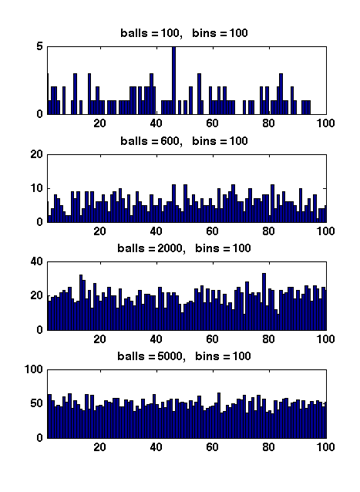}[/math] Figure 1 Due to the symmetry. All [math]\displaystyle{ X_i }[/math] have the same distribution. Apply the union bound again, [math]\displaystyle{ \begin{align} \Pr\left[\max_{1\le i\le n}X_i\ge M\right] &= \Pr\left[(X_1\ge M) \vee (X_2\ge M) \vee\cdots\vee (X_n\ge M)\right]\\ &\le n\Pr[X_1\ge M]\\ &\le n\left(\frac{e}{M}\right)^M. \end{align} }[/math] When [math]\displaystyle{ M=3\ln n/\ln\ln n }[/math], [math]\displaystyle{ \begin{align} \left(\frac{e}{M}\right)^M &= \left(\frac{e\ln\ln n}{3\ln n}\right)^{3\ln n/\ln\ln n}\\ &\lt \left(\frac{\ln\ln n}{\ln n}\right)^{3\ln n/\ln\ln n}\\ &= e^{3(\ln\ln\ln n-\ln\ln n)\ln n/\ln\ln n}\\ &= e^{-3\ln n+3\ln\ln\ln n\ln n/\ln\ln n}\\ &\le e^{-2\ln n}\\ &= \frac{1}{n^2}. \end{align} }[/math] Therefore, [math]\displaystyle{ \begin{align} \Pr\left[\max_{1\le i\le n}X_i\ge \frac{3\ln n}{\ln\ln n}\right] &\le n\left(\frac{e}{M}\right)^M &\lt \frac{1}{n}. \end{align} }[/math] [math]\displaystyle{ \square }[/math]

When [math]\displaystyle{ m\gt n }[/math], Figure 1 illustrates the results of several random experiments, which show that the distribution of the loads of bins becomes more even as the number of balls grows larger than the number of bins.

Formally, it can be proved that for [math]\displaystyle{ m=\Omega(n\log n) }[/math], with high probability, the maximum load is within [math]\displaystyle{ O\left(\frac{m}{n}\right) }[/math], which is asymptotically equal to the average load.