高级算法 (Fall 2017)/Balls into bins and Chernoff bound

Balls into Bins

Consider throwing [math]\displaystyle{ m }[/math] balls into [math]\displaystyle{ n }[/math] bins uniformly and independently at random. This is equivalent to a random mapping [math]\displaystyle{ f:[m]\to[n] }[/math]. Needless to say, random mapping is an important random model and may have many applications in Computer Science, e.g. hashing.

We are concerned with the following three questions regarding the balls into bins model:

• birthday problem: the probability that every bin contains at most one ball (the mapping is 1-1);
• coupon collector problem: the probability that every bin contains at least one ball (the mapping is on-to);
• occupancy problem: the maximum load of bins.

Birthday Problem

There are [math]\displaystyle{ m }[/math] students in the class. Assume that for each student, his/her birthday is uniformly and independently distributed over the 365 days in a years. We wonder what the probability that no two students share a birthday.

Due to the pigeonhole principle, it is obvious that for [math]\displaystyle{ m\gt 365 }[/math], there must be two students with the same birthday. Surprisingly, for any [math]\displaystyle{ m\gt 57 }[/math] this event occurs with more than 99% probability. This is called the birthday paradox. Despite the name, the birthday paradox is not a real paradox.

We can model this problem as a balls-into-bins problem. [math]\displaystyle{ m }[/math] different balls (students) are uniformly and independently thrown into 365 bins (days). More generally, let [math]\displaystyle{ n }[/math] be the number of bins. We ask for the probability of the following event [math]\displaystyle{ \mathcal{E} }[/math]

• [math]\displaystyle{ \mathcal{E} }[/math]: there is no bin with more than one balls (i.e. no two students share birthday).

We first analyze this by counting. There are totally [math]\displaystyle{ n^m }[/math] ways of assigning [math]\displaystyle{ m }[/math] balls to [math]\displaystyle{ n }[/math] bins. The number of assignments that no two balls share a bin is [math]\displaystyle{ {n\choose m}m! }[/math].

Thus the probability is given by:

[math]\displaystyle{ \begin{align} \Pr[\mathcal{E}] = \frac{{n\choose m}m!}{n^m}. \end{align} }[/math]

Recall that [math]\displaystyle{ {n\choose m}=\frac{n!}{(n-m)!m!} }[/math]. Then

[math]\displaystyle{ \begin{align} \Pr[\mathcal{E}] = \frac{{n\choose m}m!}{n^m} = \frac{n!}{n^m(n-m)!} = \frac{n}{n}\cdot\frac{n-1}{n}\cdot\frac{n-2}{n}\cdots\frac{n-(m-1)}{n} = \prod_{k=1}^{m-1}\left(1-\frac{k}{n}\right). \end{align} }[/math]

There is also a more "probabilistic" argument for the above equation. Consider again that [math]\displaystyle{ m }[/math] students are mapped to [math]\displaystyle{ n }[/math] possible birthdays uniformly at random.

The first student has a birthday for sure. The probability that the second student has a different birthday from the first student is [math]\displaystyle{ \left(1-\frac{1}{n}\right) }[/math]. Given that the first two students have different birthdays, the probability that the third student has a different birthday from the first two students is [math]\displaystyle{ \left(1-\frac{2}{n}\right) }[/math]. Continuing this on, assuming that the first [math]\displaystyle{ k-1 }[/math] students all have different birthdays, the probability that the [math]\displaystyle{ k }[/math]th student has a different birthday than the first [math]\displaystyle{ k-1 }[/math], is given by [math]\displaystyle{ \left(1-\frac{k-1}{n}\right) }[/math]. By the chain rule, the probability that all [math]\displaystyle{ m }[/math] students have different birthdays is:

[math]\displaystyle{ \begin{align} \Pr[\mathcal{E}]=\left(1-\frac{1}{n}\right)\cdot \left(1-\frac{2}{n}\right)\cdots \left(1-\frac{m-1}{n}\right) &= \prod_{k=1}^{m-1}\left(1-\frac{k}{n}\right), \end{align} }[/math]

which is the same as what we got by the counting argument.

There are several ways of analyzing this formular. Here is a convenient one: Due to Taylor's expansion, [math]\displaystyle{ e^{-k/n}\approx 1-k/n }[/math]. Then

[math]\displaystyle{ \begin{align} \prod_{k=1}^{m-1}\left(1-\frac{k}{n}\right) &\approx \prod_{k=1}^{m-1}e^{-\frac{k}{n}}\\ &= \exp\left(-\sum_{k=1}^{m-1}\frac{k}{n}\right)\\ &= e^{-m(m-1)/2n}\\ &\approx e^{-m^2/2n}. \end{align} }[/math]

The quality of this approximation is shown in the Figure.

Therefore, for [math]\displaystyle{ m=\sqrt{2n\ln \frac{1}{\epsilon}} }[/math], the probability that [math]\displaystyle{ \Pr[\mathcal{E}]\approx\epsilon }[/math].

Coupon Collector

Suppose that a chocolate company releases [math]\displaystyle{ n }[/math] different types of coupons. Each box of chocolates contains one coupon with a uniformly random type. Once you have collected all [math]\displaystyle{ n }[/math] types of coupons, you will get a prize. So how many boxes of chocolates you are expected to buy to win the prize?

The coupon collector problem can be described in the balls-into-bins model as follows. We keep throwing balls one-by-one into [math]\displaystyle{ n }[/math] bins (coupons), such that each ball is thrown into a bin uniformly and independently at random. Each ball corresponds to a box of chocolate, and each bin corresponds to a type of coupon. Thus, the number of boxes bought to collect [math]\displaystyle{ n }[/math] coupons is just the number of balls thrown until none of the [math]\displaystyle{ n }[/math] bins is empty.

Theorem

Let [math]\displaystyle{ X }[/math] be the number of balls thrown uniformly and independently to [math]\displaystyle{ n }[/math] bins until no bin is empty. Then [math]\displaystyle{ \mathbf{E}[X]=nH(n) }[/math], where [math]\displaystyle{ H(n) }[/math] is the [math]\displaystyle{ n }[/math]th harmonic number.

Proof. Let [math]\displaystyle{ X_i }[/math] be the number of balls thrown while there are exactly [math]\displaystyle{ i-1 }[/math] nonempty bins, then clearly [math]\displaystyle{ X=\sum_{i=1}^n X_i }[/math]. When there are exactly [math]\displaystyle{ i-1 }[/math] nonempty bins, throwing a ball, the probability that the number of nonempty bins increases (i.e. the ball is thrown to an empty bin) is [math]\displaystyle{ p_i=1-\frac{i-1}{n}. }[/math] [math]\displaystyle{ X_i }[/math] is the number of balls thrown to make the number of nonempty bins increases from [math]\displaystyle{ i-1 }[/math] to [math]\displaystyle{ i }[/math], i.e. the number of balls thrown until a ball is thrown to a current empty bin. Thus, [math]\displaystyle{ X_i }[/math] follows the geometric distribution, such that [math]\displaystyle{ \Pr[X_i=k]=(1-p_i)^{k-1}p_i }[/math] For a geometric random variable, [math]\displaystyle{ \mathbf{E}[X_i]=\frac{1}{p_i}=\frac{n}{n-i+1} }[/math]. Applying the linearity of expectations, [math]\displaystyle{ \begin{align} \mathbf{E}[X] &= \mathbf{E}\left[\sum_{i=1}^nX_i\right]\\ &= \sum_{i=1}^n\mathbf{E}\left[X_i\right]\\ &= \sum_{i=1}^n\frac{n}{n-i+1}\\ &= n\sum_{i=1}^n\frac{1}{i}\\ &= nH(n), \end{align} }[/math] where [math]\displaystyle{ H(n) }[/math] is the [math]\displaystyle{ n }[/math]th Harmonic number, and [math]\displaystyle{ H(n)=\ln n+O(1) }[/math]. Thus, for the coupon collectors problem, the expected number of coupons required to obtain all [math]\displaystyle{ n }[/math] types of coupons is [math]\displaystyle{ n\ln n+O(n) }[/math]. [math]\displaystyle{ \square }[/math]

---

Only knowing the expectation is not good enough. We would like to know how fast the probability decrease as a random variable deviates from its mean value.

Theorem

Let [math]\displaystyle{ X }[/math] be the number of balls thrown uniformly and independently to [math]\displaystyle{ n }[/math] bins until no bin is empty. Then [math]\displaystyle{ \Pr[X\ge n\ln n+cn]\lt e^{-c} }[/math] for any [math]\displaystyle{ c\gt 0 }[/math].

Proof. For any particular bin [math]\displaystyle{ i }[/math], the probability that bin [math]\displaystyle{ i }[/math] is empty after throwing [math]\displaystyle{ n\ln n+cn }[/math] balls is [math]\displaystyle{ \left(1-\frac{1}{n}\right)^{n\ln n+cn} \lt e^{-(\ln n+c)} =\frac{1}{ne^c}. }[/math] By the union bound, the probability that there exists an empty bin after throwing [math]\displaystyle{ n\ln n+cn }[/math] balls is [math]\displaystyle{ \Pr[X\ge n\ln n+cn] \lt n\cdot \frac{1}{ne^c} =e^{-c}. }[/math] [math]\displaystyle{ \square }[/math]

Occupancy Problem

Now we ask about the loads of bins. Assuming that [math]\displaystyle{ m }[/math] balls are uniformly and independently assigned to [math]\displaystyle{ n }[/math] bins, for [math]\displaystyle{ 1\le i\le n }[/math], let [math]\displaystyle{ X_i }[/math] be the load of the [math]\displaystyle{ i }[/math]th bin, i.e. the number of balls in the [math]\displaystyle{ i }[/math]th bin.

An easy analysis shows that for every bin [math]\displaystyle{ i }[/math], the expected load [math]\displaystyle{ \mathbf{E}[X_i] }[/math] is equal to the average load [math]\displaystyle{ m/n }[/math].

Because there are totally [math]\displaystyle{ m }[/math] balls, it is always true that [math]\displaystyle{ \sum_{i=1}^n X_i=m }[/math].

Therefore, due to the linearity of expectations,

[math]\displaystyle{ \begin{align} \sum_{i=1}^n\mathbf{E}[X_i] &= \mathbf{E}\left[\sum_{i=1}^n X_i\right] = \mathbf{E}\left[m\right] =m. \end{align} }[/math]

Because for each ball, the bin to which the ball is assigned is uniformly and independently chosen, the distributions of the loads of bins are identical. Thus [math]\displaystyle{ \mathbf{E}[X_i] }[/math] is the same for each [math]\displaystyle{ i }[/math]. Combining with the above equation, it holds that for every [math]\displaystyle{ 1\le i\le m }[/math], [math]\displaystyle{ \mathbf{E}[X_i]=\frac{m}{n} }[/math]. So the average is indeed the average!

---

Next we analyze the distribution of the maximum load. We show that when [math]\displaystyle{ m=n }[/math], i.e. [math]\displaystyle{ n }[/math] balls are uniformly and independently thrown into [math]\displaystyle{ n }[/math] bins, the maximum load is [math]\displaystyle{ O\left(\frac{\log n}{\log\log n}\right) }[/math] with high probability.

Theorem

Suppose that [math]\displaystyle{ n }[/math] balls are thrown independently and uniformly at random into [math]\displaystyle{ n }[/math] bins. For [math]\displaystyle{ 1\le i\le n }[/math], let [math]\displaystyle{ X_i }[/math] be the random variable denoting the number of balls in the [math]\displaystyle{ i }[/math]th bin. Then [math]\displaystyle{ \Pr\left[\max_{1\le i\le n}X_i \ge\frac{3\ln n}{\ln\ln n}\right] \lt \frac{1}{n}. }[/math]

Proof. Let [math]\displaystyle{ M }[/math] be an integer. Take bin 1. For any particular [math]\displaystyle{ M }[/math] balls, these [math]\displaystyle{ M }[/math] balls are all thrown to bin 1 with probability [math]\displaystyle{ (1/n)^M }[/math], and there are totally [math]\displaystyle{ {n\choose M} }[/math] distinct sets of [math]\displaystyle{ M }[/math] balls. Therefore, applying the union bound, [math]\displaystyle{ \begin{align}\Pr\left[X_1\ge M\right] &\le {n\choose M}\left(\frac{1}{n}\right)^M\\ &= \frac{n!}{M!(n-M)!n^M}\\ &= \frac{1}{M!}\cdot\frac{n(n-1)(n-2)\cdots(n-M+1)}{n^M}\\ &= \frac{1}{M!}\cdot \prod_{i=0}^{M-1}\left(1-\frac{i}{n}\right)\\ &\le \frac{1}{M!}. \end{align} }[/math] According to Stirling's approximation, [math]\displaystyle{ M!\approx \sqrt{2\pi M}\left(\frac{M}{e}\right)^M }[/math], thus [math]\displaystyle{ \frac{1}{M!}\le\left(\frac{e}{M}\right)^M. 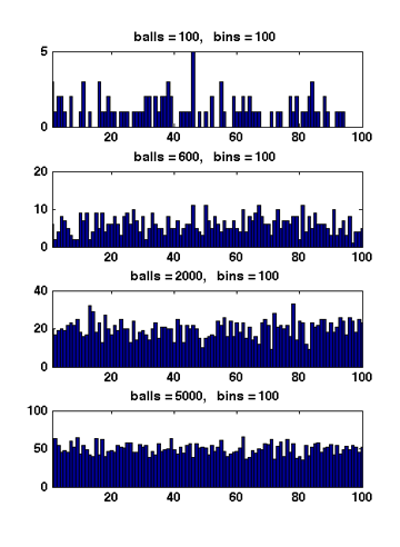}[/math] Figure 1 Due to the symmetry. All [math]\displaystyle{ X_i }[/math] have the same distribution. Apply the union bound again, [math]\displaystyle{ \begin{align} \Pr\left[\max_{1\le i\le n}X_i\ge M\right] &= \Pr\left[(X_1\ge M) \vee (X_2\ge M) \vee\cdots\vee (X_n\ge M)\right]\\ &\le n\Pr[X_1\ge M]\\ &\le n\left(\frac{e}{M}\right)^M. \end{align} }[/math] When [math]\displaystyle{ M=3\ln n/\ln\ln n }[/math], [math]\displaystyle{ \begin{align} \left(\frac{e}{M}\right)^M &= \left(\frac{e\ln\ln n}{3\ln n}\right)^{3\ln n/\ln\ln n}\\ &\lt \left(\frac{\ln\ln n}{\ln n}\right)^{3\ln n/\ln\ln n}\\ &= e^{3(\ln\ln\ln n-\ln\ln n)\ln n/\ln\ln n}\\ &= e^{-3\ln n+3\ln\ln\ln n\ln n/\ln\ln n}\\ &\le e^{-2\ln n}\\ &= \frac{1}{n^2}. \end{align} }[/math] Therefore, [math]\displaystyle{ \begin{align} \Pr\left[\max_{1\le i\le n}X_i\ge \frac{3\ln n}{\ln\ln n}\right] &\le n\left(\frac{e}{M}\right)^M &\lt \frac{1}{n}. \end{align} }[/math] [math]\displaystyle{ \square }[/math]

When [math]\displaystyle{ m\gt n }[/math], Figure 1 illustrates the results of several random experiments, which show that the distribution of the loads of bins becomes more even as the number of balls grows larger than the number of bins.

Formally, it can be proved that for [math]\displaystyle{ m=\Omega(n\log n) }[/math], with high probability, the maximum load is within [math]\displaystyle{ O\left(\frac{m}{n}\right) }[/math], which is asymptotically equal to the average load.

The Chernoff Bound

Suppose that we have a fair coin. If we toss it once, then the outcome is completely unpredictable. But if we toss it, say for 1000 times, then the number of HEADs is very likely to be around 500. This striking phenomenon, illustrated in the right figure, is called the concentration. The Chernoff bound captures the concentration of independent trials.

The Chernoff bound is also a tail bound for the sum of independent random variables which may give us exponentially sharp bounds.

Before proving the Chernoff bound, we should talk about the moment generating functions.

Moment generating functions

The more we know about the moments of a random variable [math]\displaystyle{ X }[/math], the more information we would have about [math]\displaystyle{ X }[/math]. There is a so-called moment generating function, which "packs" all the information about the moments of [math]\displaystyle{ X }[/math] into one function.

Definition

The moment generating function of a random variable [math]\displaystyle{ X }[/math] is defined as [math]\displaystyle{ \mathbf{E}\left[\mathrm{e}^{\lambda X}\right] }[/math] where [math]\displaystyle{ \lambda }[/math] is the parameter of the function.

By Taylor's expansion and the linearity of expectations,

[math]\displaystyle{ \begin{align} \mathbf{E}\left[\mathrm{e}^{\lambda X}\right] &= \mathbf{E}\left[\sum_{k=0}^\infty\frac{\lambda^k}{k!}X^k\right]\\ &=\sum_{k=0}^\infty\frac{\lambda^k}{k!}\mathbf{E}\left[X^k\right] \end{align} }[/math]

The moment generating function [math]\displaystyle{ \mathbf{E}\left[\mathrm{e}^{\lambda X}\right] }[/math] is a function of [math]\displaystyle{ \lambda }[/math].

The Chernoff bound

The Chernoff bounds are exponentially sharp tail inequalities for the sum of independent trials. The bounds are obtained by applying Markov's inequality to the moment generating function of the sum of independent trials, with some appropriate choice of the parameter [math]\displaystyle{ \lambda }[/math].

Chernoff bound (the upper tail)

Let [math]\displaystyle{ X=\sum_{i=1}^n X_i }[/math], where [math]\displaystyle{ X_1, X_2, \ldots, X_n }[/math] are independent Poisson trials. Let [math]\displaystyle{ \mu=\mathbf{E}[X] }[/math]. Then for any [math]\displaystyle{ \delta\gt 0 }[/math], [math]\displaystyle{ \Pr[X\ge (1+\delta)\mu]\le\left(\frac{e^{\delta}}{(1+\delta)^{(1+\delta)}}\right)^{\mu}. }[/math]

Proof. For any [math]\displaystyle{ \lambda\gt 0 }[/math], [math]\displaystyle{ X\ge (1+\delta)\mu }[/math] is equivalent to that [math]\displaystyle{ e^{\lambda X}\ge e^{\lambda (1+\delta)\mu} }[/math], thus [math]\displaystyle{ \begin{align} \Pr[X\ge (1+\delta)\mu] &= \Pr\left[e^{\lambda X}\ge e^{\lambda (1+\delta)\mu}\right]\\ &\le \frac{\mathbf{E}\left[e^{\lambda X}\right]}{e^{\lambda (1+\delta)\mu}}, \end{align} }[/math] where the last step follows by Markov's inequality. Computing the moment generating function [math]\displaystyle{ \mathbf{E}[e^{\lambda X}] }[/math]: [math]\displaystyle{ \begin{align} \mathbf{E}\left[e^{\lambda X}\right] &= \mathbf{E}\left[e^{\lambda \sum_{i=1}^n X_i}\right]\\ &= \mathbf{E}\left[\prod_{i=1}^n e^{\lambda X_i}\right]\\ &= \prod_{i=1}^n \mathbf{E}\left[e^{\lambda X_i}\right]. & (\mbox{for independent random variables}) \end{align} }[/math] Let [math]\displaystyle{ p_i=\Pr[X_i=1] }[/math] for [math]\displaystyle{ i=1,2,\ldots,n }[/math]. Then, [math]\displaystyle{ \mu=\mathbf{E}[X]=\mathbf{E}\left[\sum_{i=1}^n X_i\right]=\sum_{i=1}^n\mathbf{E}[X_i]=\sum_{i=1}^n p_i }[/math]. We bound the moment generating function for each individual [math]\displaystyle{ X_i }[/math] as follows. [math]\displaystyle{ \begin{align} \mathbf{E}\left[e^{\lambda X_i}\right] &= p_i\cdot e^{\lambda\cdot 1}+(1-p_i)\cdot e^{\lambda\cdot 0}\\ &= 1+p_i(e^\lambda -1)\\ &\le e^{p_i(e^\lambda-1)}, \end{align} }[/math] where in the last step we apply the Taylor's expansion so that [math]\displaystyle{ e^y\ge 1+y }[/math] where [math]\displaystyle{ y=p_i(e^\lambda-1)\ge 0 }[/math]. (By doing this, we can transform the product to the sum of [math]\displaystyle{ p_i }[/math], which is [math]\displaystyle{ \mu }[/math].) Therefore, [math]\displaystyle{ \begin{align} \mathbf{E}\left[e^{\lambda X}\right] &= \prod_{i=1}^n \mathbf{E}\left[e^{\lambda X_i}\right]\\ &\le \prod_{i=1}^n e^{p_i(e^\lambda-1)}\\ &= \exp\left(\sum_{i=1}^n p_i(e^{\lambda}-1)\right)\\ &= e^{(e^\lambda-1)\mu}. \end{align} }[/math] Thus, we have shown that for any [math]\displaystyle{ \lambda\gt 0 }[/math], [math]\displaystyle{ \begin{align} \Pr[X\ge (1+\delta)\mu] &\le \frac{\mathbf{E}\left[e^{\lambda X}\right]}{e^{\lambda (1+\delta)\mu}}\\ &\le \frac{e^{(e^\lambda-1)\mu}}{e^{\lambda (1+\delta)\mu}}\\ &= \left(\frac{e^{(e^\lambda-1)}}{e^{\lambda (1+\delta)}}\right)^\mu \end{align} }[/math]. For any [math]\displaystyle{ \delta\gt 0 }[/math], we can let [math]\displaystyle{ \lambda=\ln(1+\delta)\gt 0 }[/math] to get [math]\displaystyle{ \Pr[X\ge (1+\delta)\mu]\le\left(\frac{e^{\delta}}{(1+\delta)^{(1+\delta)}}\right)^{\mu}. }[/math] [math]\displaystyle{ \square }[/math]

The idea of the proof is actually quite clear: we apply Markov's inequality to [math]\displaystyle{ e^{\lambda X} }[/math] and for the rest, we just estimate the moment generating function [math]\displaystyle{ \mathbf{E}[e^{\lambda X}] }[/math]. To make the bound as tight as possible, we minimized the [math]\displaystyle{ \frac{e^{(e^\lambda-1)}}{e^{\lambda (1+\delta)}} }[/math] by setting [math]\displaystyle{ \lambda=\ln(1+\delta) }[/math], which can be justified by taking derivatives of [math]\displaystyle{ \frac{e^{(e^\lambda-1)}}{e^{\lambda (1+\delta)}} }[/math].

---

We then proceed to the lower tail, the probability that the random variable deviates below the mean value:

Chernoff bound (the lower tail)

Let [math]\displaystyle{ X=\sum_{i=1}^n X_i }[/math], where [math]\displaystyle{ X_1, X_2, \ldots, X_n }[/math] are independent Poisson trials. Let [math]\displaystyle{ \mu=\mathbf{E}[X] }[/math]. Then for any [math]\displaystyle{ 0\lt \delta\lt 1 }[/math], [math]\displaystyle{ \Pr[X\le (1-\delta)\mu]\le\left(\frac{e^{-\delta}}{(1-\delta)^{(1-\delta)}}\right)^{\mu}. }[/math]

Proof. For any [math]\displaystyle{ \lambda\lt 0 }[/math], by the same analysis as in the upper tail version, [math]\displaystyle{ \begin{align} \Pr[X\le (1-\delta)\mu] &= \Pr\left[e^{\lambda X}\ge e^{\lambda (1-\delta)\mu}\right]\\ &\le \frac{\mathbf{E}\left[e^{\lambda X}\right]}{e^{\lambda (1-\delta)\mu}}\\ &\le \left(\frac{e^{(e^\lambda-1)}}{e^{\lambda (1-\delta)}}\right)^\mu. \end{align} }[/math] For any [math]\displaystyle{ 0\lt \delta\lt 1 }[/math], we can let [math]\displaystyle{ \lambda=\ln(1-\delta)\lt 0 }[/math] to get [math]\displaystyle{ \Pr[X\ge (1-\delta)\mu]\le\left(\frac{e^{-\delta}}{(1-\delta)^{(1-\delta)}}\right)^{\mu}. }[/math] [math]\displaystyle{ \square }[/math]

Useful forms of the Chernoff bounds

Some useful special forms of the bounds can be derived directly from the above general forms of the bounds. We now know better why we say that the bounds are exponentially sharp.

Useful forms of the Chernoff bound

Let [math]\displaystyle{ X=\sum_{i=1}^n X_i }[/math], where [math]\displaystyle{ X_1, X_2, \ldots, X_n }[/math] are independent Poisson trials. Let [math]\displaystyle{ \mu=\mathbf{E}[X] }[/math]. Then 1. for [math]\displaystyle{ 0\lt \delta\le 1 }[/math], [math]\displaystyle{ \Pr[X\ge (1+\delta)\mu]\lt \exp\left(-\frac{\mu\delta^2}{3}\right); }[/math] [math]\displaystyle{ \Pr[X\le (1-\delta)\mu]\lt \exp\left(-\frac{\mu\delta^2}{2}\right); }[/math] 2. for [math]\displaystyle{ t\ge 2e\mu }[/math], [math]\displaystyle{ \Pr[X\ge t]\le 2^{-t}. }[/math]

Proof. To obtain the bounds in (1), we need to show that for [math]\displaystyle{ 0\lt \delta\lt 1 }[/math], [math]\displaystyle{ \frac{e^{\delta}}{(1+\delta)^{(1+\delta)}}\le e^{-\delta^2/3} }[/math] and [math]\displaystyle{ \frac{e^{-\delta}}{(1-\delta)^{(1-\delta)}}\le e^{-\delta^2/2} }[/math]. We can verify both inequalities by standard analysis techniques. To obtain the bound in (2), let [math]\displaystyle{ t=(1+\delta)\mu }[/math]. Then [math]\displaystyle{ \delta=t/\mu-1\ge 2e-1 }[/math]. Hence, [math]\displaystyle{ \begin{align} \Pr[X\ge(1+\delta)\mu] &\le \left(\frac{e^\delta}{(1+\delta)^{(1+\delta)}}\right)^\mu\\ &\le \left(\frac{e}{1+\delta}\right)^{(1+\delta)\mu}\\ &\le \left(\frac{e}{2e}\right)^t\\ &\le 2^{-t} \end{align} }[/math] [math]\displaystyle{ \square }[/math]

Applications to balls-into-bins

Throwing [math]\displaystyle{ m }[/math] balls uniformly and independently to [math]\displaystyle{ n }[/math] bins, what is the maximum load of all bins with high probability? In the last class, we gave an analysis of this problem by using a counting argument.

Now we give a more "advanced" analysis by using Chernoff bounds.

For any [math]\displaystyle{ i\in[n] }[/math] and [math]\displaystyle{ j\in[m] }[/math], let [math]\displaystyle{ X_{ij} }[/math] be the indicator variable for the event that ball [math]\displaystyle{ j }[/math] is thrown to bin [math]\displaystyle{ i }[/math]. Obviously

[math]\displaystyle{ \mathbf{E}[X_{ij}]=\Pr[\mbox{ball }j\mbox{ is thrown to bin }i]=\frac{1}{n} }[/math]

Let [math]\displaystyle{ Y_i=\sum_{j\in[m]}X_{ij} }[/math] be the load of bin [math]\displaystyle{ i }[/math].

Then the expected load of bin [math]\displaystyle{ i }[/math] is

[math]\displaystyle{ (*)\qquad \mu=\mathbf{E}[Y_i]=\mathbf{E}\left[\sum_{j\in[m]}X_{ij}\right]=\sum_{j\in[m]}\mathbf{E}[X_{ij}]=m/n. }[/math]

For the case [math]\displaystyle{ m=n }[/math], it holds that [math]\displaystyle{ \mu=1 }[/math]

Note that [math]\displaystyle{ Y_i }[/math] is a sum of [math]\displaystyle{ m }[/math] mutually independent indicator variable. Applying Chernoff bound, for any particular bin [math]\displaystyle{ i\in[n] }[/math],

[math]\displaystyle{ \Pr[Y_i\gt (1+\delta)\mu] \le \left(\frac{e^{\delta}}{(1+\delta)^{1+\delta}}\right)^\mu. }[/math]

The [math]\displaystyle{ m=n }[/math] case

When [math]\displaystyle{ m=n }[/math], [math]\displaystyle{ \mu=1 }[/math]. Write [math]\displaystyle{ c=1+\delta }[/math]. The above bound can be written as

[math]\displaystyle{ \Pr[Y_i\gt c] \le \frac{e^{c-1}}{c^c}. }[/math]

Let [math]\displaystyle{ c=\frac{e\ln n}{\ln\ln n} }[/math], we evaluate [math]\displaystyle{ \frac{e^{c-1}}{c^c} }[/math] by taking logarithm to its reciprocal.

[math]\displaystyle{ \begin{align} \ln\left(\frac{c^c}{e^{c-1}}\right) &= c\ln c-c+1\\ &= c(\ln c-1)+1\\ &= \frac{e\ln n}{\ln\ln n}\left(\ln\ln n-\ln\ln\ln n\right)+1\\ &\ge \frac{e\ln n}{\ln\ln n}\cdot\frac{2}{e}\ln\ln n+1\\ &\ge 2\ln n. \end{align} }[/math]

Thus,

[math]\displaystyle{ \Pr\left[Y_i\gt \frac{e\ln n}{\ln\ln n}\right] \le \frac{1}{n^2}. }[/math]

Applying the union bound, the probability that there exists a bin with load [math]\displaystyle{ \gt 12\ln n }[/math] is

[math]\displaystyle{ n\cdot \Pr\left[Y_1\gt \frac{e\ln n}{\ln\ln n}\right] \le \frac{1}{n} }[/math].

Therefore, for [math]\displaystyle{ m=n }[/math], with high probability, the maximum load is [math]\displaystyle{ O\left(\frac{e\ln n}{\ln\ln n}\right) }[/math].

The [math]\displaystyle{ m\gt \ln n }[/math] case

When [math]\displaystyle{ m\ge n\ln n }[/math], then according to [math]\displaystyle{ (*) }[/math], [math]\displaystyle{ \mu=\frac{m}{n}\ge \ln n }[/math]

We can apply an easier form of the Chernoff bounds,

[math]\displaystyle{ \Pr[Y_i\ge 2e\mu]\le 2^{-2e\mu}\le 2^{-2e\ln n}\lt \frac{1}{n^2}. }[/math]

By the union bound, the probability that there exists a bin with load [math]\displaystyle{ \ge 2e\frac{m}{n} }[/math] is,

[math]\displaystyle{ n\cdot \Pr\left[Y_1\gt 2e\frac{m}{n}\right] = n\cdot \Pr\left[Y_1\gt 2e\mu\right]\le \frac{1}{n} }[/math].

Therefore, for [math]\displaystyle{ m\ge n\ln n }[/math], with high probability, the maximum load is [math]\displaystyle{ O\left(\frac{m}{n}\right) }[/math].