随机算法 (Spring 2013)/Random Variables and Expectations: Difference between revisions
imported>Etone |
imported>Etone |
||
| (4 intermediate revisions by the same user not shown) | |||
| Line 7: | Line 7: | ||
:<math>\Pr[X=x]=\Pr(\{a\in\Omega\mid X(a)=x\})</math>. | :<math>\Pr[X=x]=\Pr(\{a\in\Omega\mid X(a)=x\})</math>. | ||
The independence can also be defined for variables: | The independence can also be defined for variables: | ||
{{Theorem | {{Theorem | ||
| Line 78: | Line 77: | ||
}} | }} | ||
There is also a '''law of total expectation'''. | There is also a '''law of total expectation'''. | ||
{{Theorem | {{Theorem | ||
| Line 192: | Line 190: | ||
Therefore, for an arbitrary input <math>S</math> of <math>n</math> numbers, the expected number of comparisons taken by RandQSort to sort <math>S</math> is <math>\mathrm{O}(n\log n)</math>. | Therefore, for an arbitrary input <math>S</math> of <math>n</math> numbers, the expected number of comparisons taken by RandQSort to sort <math>S</math> is <math>\mathrm{O}(n\log n)</math>. | ||
= Distributions of Coin Flips = | |||
We introduce several important distributions induced by independent coin flips (independent probabilistic experiments), including: Bernoulli trial, geometric distribution, binomial distribution. | |||
==Bernoulli trial (Bernoulli distribution)== | |||
Bernoulli trial describes the probability distribution of a single (biased) coin flip. Suppose that we flip a (biased) coin where the probability of HEADS is <math>p</math>. Let <math>X</math> be the 0-1 random variable which indicates whether the result is HEADS. We say that <math>X</math> follows the Bernoulli distribution with parameter <math>p</math>. Formally, | |||
:<math>\begin{align} | |||
X | |||
&= | |||
\begin{cases} | |||
1 & \text{with probability }p\ | |||
0 & \text{with probability }1-p | |||
\end{cases} | |||
\end{align}</math>. | |||
==Geometric distribution== | |||
Suppose we flip the same coin repeatedly until HEADS appears, where each coin flip is independent and follows the Bernoulli distribution with parameter <math>p</math>. Let <math>X</math> be the random variable denoting the total number of coin flips. Then <math>X</math> has the geometric distribution with parameter <math>p</math>. Formally, <math>\Pr[X=k]=(1-p)^{k-1}p</math>. | |||
For geometric <math>X</math>, <math>\mathbf{E}[X]=\frac{1}{p}</math>. This can be verified by directly computing <math>\mathbf{E}[X]</math> by the definition of expectations. There is also a smarter way of computing <math>\mathbf{E}[X]</math>, by using indicators and the linearity of expectations. For <math>k=0, 1, 2, \ldots</math>, let <math>Y_k</math> be the 0-1 random variable such that <math>Y_k=1</math> if and only if none of the first <math>k</math> coin flipings are HEADS, thus <math>\mathbf{E}[Y_k]=\Pr[Y_k=1]=(1-p)^{k}</math>. A key observation is that <math>X=\sum_{k=0}^\infty Y_k</math>. Thus, due to the linearity of expectations, | |||
:<math> | |||
\begin{align} | |||
\mathbf{E}[X] | |||
= | |||
\mathbf{E}\left[\sum_{k=0}^\infty Y_k\right] | |||
= | |||
\sum_{k=0}^\infty \mathbf{E}[Y_k] | |||
= | |||
\sum_{k=0}^\infty (1-p)^k | |||
= | |||
\frac{1}{1-(1-p)} | |||
=\frac{1}{p}. | |||
\end{align} | |||
</math> | |||
==Binomial distribution== | |||
Suppose we flip the same (biased) coin for <math>n</math> times, where each coin flip is independent and follows the Bernoulli distribution with parameter <math>p</math>. Let <math>X</math> be the number of HEADS. Then <math>X</math> has the binomial distribution with parameters <math>n</math> and <math>p</math>. Formally, <math>\Pr[X=k]={n\choose k}p^k(1-p)^{n-k}</math>. | |||
A binomial random variable <math>X</math> with parameters <math>n</math> and <math>p</math> is usually denoted by <math>B(n,p)</math>. | |||
As we saw above, by applying the linearity of expectations, it is easy to show that <math>\mathbf{E}[X]=np</math> for an <math>X=B(n,p)</math>. | |||
=Balls into Bins= | |||
== Birthday Problem== | |||
There are <math>m</math> students in the class. Assume that for each student, his/her birthday is uniformly and independently distributed over the 365 days in a years. We wonder what the probability that no two students share a birthday. | |||
Due to the [http://en.wikipedia.org/wiki/Pigeonhole_principle pigeonhole principle], it is obvious that for <math>m>365</math>, there must be two students with the same birthday. Surprisingly, for any <math>m>57</math> this event occurs with more than 99% probability. This is called the [http://en.wikipedia.org/wiki/Birthday_problem '''birthday paradox''']. Despite the name, the birthday paradox is not a real paradox. | |||
We can model this problem as a balls-into-bins problem. <math>m</math> different balls (students) are uniformly and independently thrown into 365 bins (days). More generally, let <math>n</math> be the number of bins. We ask for the probability of the following event <math>\mathcal{E}</math> | |||
* <math>\mathcal{E}</math>: there is no bin with more than one balls (i.e. no two students share birthday). | |||
We first analyze this by counting. There are totally <math>n^m</math> ways of assigning <math>m</math> balls to <math>n</math> bins. The number of assignments that no two balls share a bin is <math>{n\choose m}m!</math>. | |||
Thus the probability is given by: | |||
:<math>\begin{align} | |||
\Pr[\mathcal{E}] | |||
= | |||
\frac{{n\choose m}m!}{n^m}. | |||
\end{align} | |||
</math> | |||
Recall that <math>{n\choose m}=\frac{n!}{(n-m)!m!}</math>. Then | |||
:<math>\begin{align} | |||
\Pr[\mathcal{E}] | |||
= | |||
\frac{{n\choose m}m!}{n^m} | |||
= | |||
\frac{n!}{n^m(n-m)!} | |||
= | |||
\frac{n}{n}\cdot\frac{n-1}{n}\cdot\frac{n-2}{n}\cdots\frac{n-(m-1)}{n} | |||
= | |||
\prod_{k=1}^{m-1}\left(1-\frac{k}{n}\right). | |||
\end{align} | |||
</math> | |||
There is also a more "probabilistic" argument for the above equation. To be rigorous, we need the following theorem, which holds generally and is very useful for computing the AND of many events. | |||
:::{|border="1" | |||
|By the definition of conditional probability, <math>\Pr[A\mid B]=\frac{\Pr[A\wedge B]}{\Pr[B]}</math>. Thus, <math>\Pr[A\wedge B] =\Pr[B]\cdot\Pr[A\mid B]</math>. This hints us that we can compute the probability of the AND of events by conditional probabilities. Formally, we have the following theorem: | |||
'''Theorem:''' | |||
:Let <math>\mathcal{E}_1, \mathcal{E}_2, \ldots, \mathcal{E}_n</math> be any <math>n</math> events. Then | |||
::<math>\begin{align} | |||
\Pr\left[\bigwedge_{i=1}^n\mathcal{E}_i\right] | |||
&= | |||
\prod_{k=1}^n\Pr\left[\mathcal{E}_k \mid \bigwedge_{i<k}\mathcal{E}_i\right]. | |||
\end{align}</math> | |||
'''Proof:''' It holds that <math>\Pr[A\wedge B] =\Pr[B]\cdot\Pr[A\mid B]</math>. Thus, let <math>A=\mathcal{E}_n</math> and <math>B=\mathcal{E}_1\wedge\mathcal{E}_2\wedge\cdots\wedge\mathcal{E}_{n-1}</math>, then | |||
:<math>\begin{align} | |||
\Pr[\mathcal{E}_1\wedge\mathcal{E}_2\wedge\cdots\wedge\mathcal{E}_n] | |||
&= | |||
\Pr[\mathcal{E}_1\wedge\mathcal{E}_2\wedge\cdots\wedge\mathcal{E}_{n-1}]\cdot\Pr\left[\mathcal{E}_n\mid \bigwedge_{i<n}\mathcal{E}_i\right]. | |||
\end{align} | |||
</math> | |||
Recursively applying this equation to <math>\Pr[\mathcal{E}_1\wedge\mathcal{E}_2\wedge\cdots\wedge\mathcal{E}_{n-1}]</math> until there is only <math>\mathcal{E}_1</math> left, the theorem is proved. <math>\square</math> | |||
|} | |||
Now we are back to the probabilistic analysis of the birthday problem, with a general setting of <math>m</math> students and <math>n</math> possible birthdays (imagine that we live in a planet where a year has <math>n</math> days). | |||
The first student has a birthday (of course!). The probability that the second student has a different birthday is <math>\left(1-\frac{1}{n}\right)</math>. Given that the first two students have different birthdays, the probability that the third student has a different birthday from the first two is <math>\left(1-\frac{2}{n}\right)</math>. Continuing this on, assuming that the first <math>k-1</math> students all have different birthdays, the probability that the <math>k</math>th student has a different birthday than the first <math>k-1</math>, is given by <math>\left(1-\frac{k-1}{n}\right)</math>. So the probability that all <math>m</math> students have different birthdays is the product of all these conditional probabilities: | |||
:<math>\begin{align} | |||
\Pr[\mathcal{E}]=\left(1-\frac{1}{n}\right)\cdot \left(1-\frac{2}{n}\right)\cdots \left(1-\frac{m-1}{n}\right) | |||
&= | |||
\prod_{k=1}^{m-1}\left(1-\frac{k}{n}\right), | |||
\end{align} | |||
</math> | |||
which is the same as what we got by the counting argument. | |||
[[File:Birthday.png|border|450px|right]] | |||
There are several ways of analyzing this formular. Here is a convenient one: Due to [http://en.wikipedia.org/wiki/Taylor_series Taylor's expansion], <math>e^{-k/n}\approx 1-k/n</math>. Then | |||
:<math>\begin{align} | |||
\prod_{k=1}^{m-1}\left(1-\frac{k}{n}\right) | |||
&\approx | |||
\prod_{k=1}^{m-1}e^{-\frac{k}{n}}\ | |||
&= | |||
\exp\left(-\sum_{k=1}^{m-1}\frac{k}{n}\right)\ | |||
&= | |||
e^{-m(m-1)/2n}\ | |||
&\approx | |||
e^{-m^2/2n}. | |||
\end{align}</math> | |||
The quality of this approximation is shown in the Figure. | |||
Therefore, for <math>m=\sqrt{2n\ln \frac{1}{\epsilon}}</math>, the probability that <math>\Pr[\mathcal{E}]\approx\epsilon</math>. | |||
==Coupon Collector == | |||
Suppose that a chocolate company releases <math>n</math> different types of coupons. Each box of chocolates contains one coupon with a uniformly random type. Once you have collected all <math>n</math> types of coupons, you will get a prize. So how many boxes of chocolates you are expected to buy to win the prize? | |||
The coupon collector problem can be described in the balls-into-bins model as follows. We keep throwing balls one-by-one into <math>n</math> bins (coupons), such that each ball is thrown into a bin uniformly and independently at random. Each ball corresponds to a box of chocolate, and each bin corresponds to a type of coupon. Thus, the number of boxes bought to collect <math>n</math> coupons is just the number of balls thrown until none of the <math>n</math> bins is empty. | |||
{{Theorem | |||
|Theorem| | |||
:Let <math>X</math> be the number of balls thrown uniformly and independently to <math>n</math> bins until no bin is empty. Then <math>\mathbf{E}[X]=nH(n)</math>, where <math>H(n)</math> is the <math>n</math>th harmonic number. | |||
}} | |||
{{Proof| Let <math>X_i</math> be the number of balls thrown while there are ''exactly'' <math>i-1</math> nonempty bins, then clearly <math>X=\sum_{i=1}^n X_i</math>. | |||
When there are exactly <math>i-1</math> nonempty bins, throwing a ball, the probability that the number of nonempty bins increases (i.e. the ball is thrown to an empty bin) is | |||
:<math>p_i=1-\frac{i-1}{n}. | |||
</math> | |||
<math>X_i</math> is the number of balls thrown to make the number of nonempty bins increases from <math>i-1</math> to <math>i</math>, i.e. the number of balls thrown until a ball is thrown to a current empty bin. Thus, <math>X_i</math> follows the [http://en.wikipedia.org/wiki/Geometric_distribution geometric distribution], such that | |||
:<math>\Pr[X_i=k]=(1-p_i)^{k-1}p_i</math> | |||
For a geometric random variable, <math>\mathbf{E}[X_i]=\frac{1}{p_i}=\frac{n}{n-i+1}</math>. | |||
Applying the linearity of expectations, | |||
:<math> | |||
\begin{align} | |||
\mathbf{E}[X] | |||
&= | |||
\mathbf{E}\left[\sum_{i=1}^nX_i\right]\ | |||
&= | |||
\sum_{i=1}^n\mathbf{E}\left[X_i\right]\ | |||
&= | |||
\sum_{i=1}^n\frac{n}{n-i+1}\ | |||
&= | |||
n\sum_{i=1}^n\frac{1}{i}\ | |||
&= | |||
nH(n), | |||
\end{align} | |||
</math> | |||
where <math>H(n)</math> is the <math>n</math>th Harmonic number, and <math>H(n)=\ln n+O(1)</math>. Thus, for the coupon collectors problem, the expected number of coupons required to obtain all <math>n</math> types of coupons is <math>n\ln n+O(n)</math>. | |||
}} | |||
---- | |||
Only knowing the expectation is not good enough. We would like to know how fast the probability decrease as a random variable deviates from its mean value. | |||
{{Theorem | |||
|Theorem| | |||
:Let <math>X</math> be the number of balls thrown uniformly and independently to <math>n</math> bins until no bin is empty. Then <math>\Pr[X\ge n\ln n+cn]<e^{-c}</math> for any <math>c>0</math>. | |||
}} | |||
{{Proof| For any particular bin <math>i</math>, the probability that bin <math>i</math> is empty after throwing <math>n\ln n+cn</math> balls is | |||
:<math>\left(1-\frac{1}{n}\right)^{n\ln n+cn} | |||
< e^{-(\ln n+c)} | |||
=\frac{1}{ne^c}. | |||
</math> | |||
By the union bound, the probability that there exists an empty bin after throwing <math>n\ln n+cn</math> balls is | |||
:<math> | |||
\Pr[X\ge n\ln n+cn] | |||
< n\cdot \frac{1}{ne^c} | |||
=e^{-c}. | |||
</math> | |||
}} | |||
== Occupancy Problem == | |||
Now we ask about the loads of bins. Assuming that <math>m</math> balls are uniformly and independently assigned to <math>n</math> bins, for <math>1\le i\le n</math>, let <math>X_i</math> be the '''load''' of the <math>i</math>th bin, i.e. the number of balls in the <math>i</math>th bin. | |||
An easy analysis shows that for every bin <math>i</math>, the expected load <math>\mathbf{E}[X_i]</math> is equal to the average load <math>m/n</math>. | |||
Because there are totally <math>m</math> balls, it is always true that <math>\sum_{i=1}^n X_i=m</math>. | |||
Therefore, due to the linearity of expectations, | |||
:<math>\begin{align} | |||
\sum_{i=1}^n\mathbf{E}[X_i] | |||
&= | |||
\mathbf{E}\left[\sum_{i=1}^n X_i\right] | |||
= | |||
\mathbf{E}\left[m\right] | |||
=m. | |||
\end{align}</math> | |||
Because for each ball, the bin to which the ball is assigned is uniformly and independently chosen, the distributions of the loads of bins are identical. Thus <math>\mathbf{E}[X_i]</math> is the same for each <math>i</math>. Combining with the above equation, it holds that for every <math>1\le i\le m</math>, <math>\mathbf{E}[X_i]=\frac{m}{n}</math>. So the average is indeed the average! | |||
---- | |||
Next we analyze the distribution of the maximum load. We show that when <math>m=n</math>, i.e. <math>n</math> balls are uniformly and independently thrown into <math>n</math> bins, the maximum load is <math>O\left(\frac{\log n}{\log\log n}\right)</math> with high probability. | |||
{{Theorem | |||
|Theorem| | |||
:Suppose that <math>n</math> balls are thrown independently and uniformly at random into <math>n</math> bins. For <math>1\le i\le n</math>, let <math>X_i</math> be the random variable denoting the number of balls in the <math>i</math>th bin. Then | |||
::<math>\Pr\left[\max_{1\le i\le n}X_i \ge\frac{3\ln n}{\ln\ln n}\right] <\frac{1}{n}.</math> | |||
}} | |||
{{Proof| Let <math>M</math> be an integer. Take bin 1. For any particular <math>M</math> balls, these <math>M</math> balls are all thrown to bin 1 with probability <math>(1/n)^M</math>, and there are totally <math>{n\choose M}</math> distinct sets of <math>M</math> balls. Therefore, applying the union bound, | |||
:<math>\begin{align}\Pr\left[X_1\ge M\right] | |||
&\le | |||
{n\choose M}\left(\frac{1}{n}\right)^M\ | |||
&= | |||
\frac{n!}{M!(n-M)!n^M}\ | |||
&= | |||
\frac{1}{M!}\cdot\frac{n(n-1)(n-2)\cdots(n-M+1)}{n^M}\ | |||
&= | |||
\frac{1}{M!}\cdot \prod_{i=0}^{M-1}\left(1-\frac{i}{n}\right)\ | |||
&\le \frac{1}{M!}. | |||
\end{align}</math> | |||
According to [http://en.wikipedia.org/wiki/Stirling's_approximation Stirling's approximation], <math>M!\approx \sqrt{2\pi M}\left(\frac{M}{e}\right)^M</math>, thus | |||
:<math>\frac{1}{M!}\le\left(\frac{e}{M}\right)^M.</math> | |||
[[file:Balls2bins.png|frame|Figure 1]] | |||
Due to the symmetry. All <math>X_i</math> have the same distribution. | |||
Apply the union bound again, | |||
:<math>\begin{align} | |||
\Pr\left[\max_{1\le i\le n}X_i\ge M\right] | |||
&= | |||
\Pr\left[(X_1\ge M) \vee (X_2\ge M) \vee\cdots\vee (X_n\ge M)\right]\ | |||
&\le | |||
n\Pr[X_1\ge M]\ | |||
&\le n\left(\frac{e}{M}\right)^M. | |||
\end{align} | |||
</math> | |||
When <math>M=3\ln n/\ln\ln n</math>, | |||
:<math>\begin{align} | |||
\left(\frac{e}{M}\right)^M | |||
&= | |||
\left(\frac{e\ln\ln n}{3\ln n}\right)^{3\ln n/\ln\ln n}\ | |||
&< | |||
\left(\frac{\ln\ln n}{\ln n}\right)^{3\ln n/\ln\ln n}\ | |||
&= | |||
e^{3(\ln\ln\ln n-\ln\ln n)\ln n/\ln\ln n}\ | |||
&= | |||
e^{-3\ln n+3\ln\ln\ln n\ln n/\ln\ln n}\ | |||
&\le | |||
e^{-2\ln n}\ | |||
&= | |||
\frac{1}{n^2}. | |||
\end{align} | |||
</math> | |||
Therefore, | |||
:<math>\begin{align} | |||
\Pr\left[\max_{1\le i\le n}X_i\ge \frac{3\ln n}{\ln\ln n}\right] | |||
&\le n\left(\frac{e}{M}\right)^M | |||
&< \frac{1}{n}. | |||
\end{align} | |||
</math> | |||
}} | |||
When <math>m>n</math>, Figure 1 illustrates the results of several random experiments, which show that the distribution of the loads of bins becomes more even as the number of balls grows larger than the number of bins. | |||
Formally, it can be proved that for <math>m=\Omega(n\log n)</math>, with high probability, the maximum load is within <math>O\left(\frac{m}{n}\right)</math>, which is asymptotically equal to the average load. | |||
Latest revision as of 10:33, 11 March 2013
Random Variable
Definition (random variable) - A random variable
- A random variable
For a random variable
The independence can also be defined for variables:
Definition (Independent variables) - Two random variables
- for all values
- Two random variables
Note that in probability theory, the "mutual independence" is not equivalent with "pair-wise independence", which we will learn in the future.
Expectation
Let
Definition (Expectation) - The expectation of a discrete random variable
- where the summation is over all values
- The expectation of a discrete random variable
Linearity of Expectation
Perhaps the most useful property of expectation is its linearity.
Theorem (Linearity of Expectations) - For any discrete random variables
- For any discrete random variables
Proof. By the definition of the expectations, it is easy to verify that (try to prove by yourself): for any discrete random variables
The theorem follows by induction.
The linearity of expectation gives an easy way to compute the expectation of a random variable if the variable can be written as a sum.
- Example
- Supposed that we have a biased coin that the probability of HEADs is
- It looks straightforward that it must be np, but how can we prove it? Surely we can apply the definition of expectation to compute the expectation with brute force. A more convenient way is by the linearity of expectations: Let
The real power of the linearity of expectations is that it does not require the random variables to be independent, thus can be applied to any set of random variables. For example:
However, do not exaggerate this power!
- For an arbitrary function
- For variances, the equation
Conditional Expectation
Conditional expectation can be accordingly defined:
Definition (conditional expectation) - For random variables
- where the summation is taken over the range of
- For random variables
There is also a law of total expectation.
Theorem (law of total expectation) - Let
- Let
Random Quicksort
Given as input a set
- if
- pick an
- partition
- recursively sort
- pick an
The time complexity of this sorting algorithm is measured by the number of comparisons.
For the deterministic quicksort algorithm, the pivot is picked from a fixed position (e.g. the first number in the array). The worst-case time complexity in terms of number of comparisons is
We consider the following randomized version of the quicksort.
- if
- uniformly pick a random
- partition
- recursively sort
- uniformly pick a random
Analysis of Random Quicksort
Our goal is to analyze the expected number of comparisons during an execution of RandQSort with an arbitrary input
Let
Elements
Observation 1: Every pair of
Therefore the sum of
By the definition of expectation and
We are going to bound this probability.
Observation 2:
This is easy to verify: just check the algorithm. The next one is a bit complicated.
Observation 3: If
We can verify this by induction. Initially,
Combining Observation 2 and 3, we have:
Observation 4:
And,
Observation 5: Every one of
This is because the Random Quicksort chooses the pivot uniformly at random.
Observation 4 and 5 together imply:
| Remark: Perhaps you feel confused about the above argument. You may ask: "The algorithm chooses pivots for many times during the execution. Why in the above argument, it looks like the pivot is chosen only once?" Good question! Let's see what really happens by looking closely.
For any pair Formally, let The conditional probability rules out the irrelevant events in a probabilistic argument. |
Summing all up:
Therefore, for an arbitrary input
Distributions of Coin Flips
We introduce several important distributions induced by independent coin flips (independent probabilistic experiments), including: Bernoulli trial, geometric distribution, binomial distribution.
Bernoulli trial (Bernoulli distribution)
Bernoulli trial describes the probability distribution of a single (biased) coin flip. Suppose that we flip a (biased) coin where the probability of HEADS is
Geometric distribution
Suppose we flip the same coin repeatedly until HEADS appears, where each coin flip is independent and follows the Bernoulli distribution with parameter
For geometric
Binomial distribution
Suppose we flip the same (biased) coin for
A binomial random variable
As we saw above, by applying the linearity of expectations, it is easy to show that
Balls into Bins
Birthday Problem
There are
Due to the pigeonhole principle, it is obvious that for
We can model this problem as a balls-into-bins problem.
We first analyze this by counting. There are totally
Thus the probability is given by:
Recall that
There is also a more "probabilistic" argument for the above equation. To be rigorous, we need the following theorem, which holds generally and is very useful for computing the AND of many events.
By the definition of conditional probability, Theorem:
- Let
Proof: It holds that
Recursively applying this equation to
- Let
Now we are back to the probabilistic analysis of the birthday problem, with a general setting of
The first student has a birthday (of course!). The probability that the second student has a different birthday is
which is the same as what we got by the counting argument.

There are several ways of analyzing this formular. Here is a convenient one: Due to Taylor's expansion,
The quality of this approximation is shown in the Figure.
Therefore, for
Coupon Collector
Suppose that a chocolate company releases
The coupon collector problem can be described in the balls-into-bins model as follows. We keep throwing balls one-by-one into
Theorem - Let
- Let
Proof. Let When there are exactly
For a geometric random variable,
Applying the linearity of expectations,
where
Only knowing the expectation is not good enough. We would like to know how fast the probability decrease as a random variable deviates from its mean value.
Theorem - Let
- Let
Proof. For any particular bin By the union bound, the probability that there exists an empty bin after throwing
Occupancy Problem
Now we ask about the loads of bins. Assuming that
An easy analysis shows that for every bin
Because there are totally
Therefore, due to the linearity of expectations,
Because for each ball, the bin to which the ball is assigned is uniformly and independently chosen, the distributions of the loads of bins are identical. Thus
Next we analyze the distribution of the maximum load. We show that when
Theorem - Suppose that
- Suppose that
Proof. Let According to Stirling's approximation,
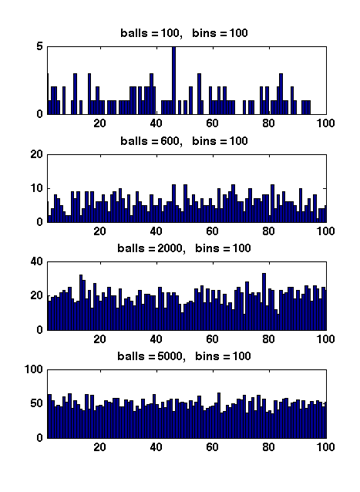
Figure 1 Due to the symmetry. All
When
Therefore,

When
Formally, it can be proved that for