高级算法 (Fall 2022)/Balls into bins

Balls into Bins

Consider throwing [math]\displaystyle{ m }[/math] balls into [math]\displaystyle{ n }[/math] bins uniformly and independently at random. This is equivalent to a random mapping [math]\displaystyle{ f:[m]\to[n] }[/math]. Needless to say, random mapping is an important random model and may have many applications in Computer Science, e.g. hashing.

We are concerned with the following three questions regarding the balls into bins model:

• birthday problem: the probability that every bin contains at most one ball (the mapping is 1-1);
• coupon collector problem: the probability that every bin contains at least one ball (the mapping is on-to);
• occupancy problem: the maximum load of bins.

Birthday Problem

There are [math]\displaystyle{ m }[/math] students in the class. Assume that for each student, his/her birthday is uniformly and independently distributed over the 365 days in a years. We wonder what the probability that no two students share a birthday.

Due to the pigeonhole principle, it is obvious that for [math]\displaystyle{ m\gt 365 }[/math], there must be two students with the same birthday. Surprisingly, for any [math]\displaystyle{ m\gt 57 }[/math] this event occurs with more than 99% probability. This is called the birthday paradox. Despite the name, the birthday paradox is not a real paradox.

We can model this problem as a balls-into-bins problem. [math]\displaystyle{ m }[/math] different balls (students) are uniformly and independently thrown into 365 bins (days). More generally, let [math]\displaystyle{ n }[/math] be the number of bins. We ask for the probability of the following event [math]\displaystyle{ \mathcal{E} }[/math]

• [math]\displaystyle{ \mathcal{E} }[/math]: there is no bin with more than one balls (i.e. no two students share birthday).

We first analyze this by counting. There are totally [math]\displaystyle{ n^m }[/math] ways of assigning [math]\displaystyle{ m }[/math] balls to [math]\displaystyle{ n }[/math] bins. The number of assignments that no two balls share a bin is [math]\displaystyle{ {n\choose m}m! }[/math].

Thus the probability is given by:

[math]\displaystyle{ \begin{align} \Pr[\mathcal{E}] = \frac{{n\choose m}m!}{n^m}. \end{align} }[/math]

Recall that [math]\displaystyle{ {n\choose m}=\frac{n!}{(n-m)!m!} }[/math]. Then

[math]\displaystyle{ \begin{align} \Pr[\mathcal{E}] = \frac{{n\choose m}m!}{n^m} = \frac{n!}{n^m(n-m)!} = \frac{n}{n}\cdot\frac{n-1}{n}\cdot\frac{n-2}{n}\cdots\frac{n-(m-1)}{n} = \prod_{k=1}^{m-1}\left(1-\frac{k}{n}\right). \end{align} }[/math]

There is also a more "probabilistic" argument for the above equation. Consider again that [math]\displaystyle{ m }[/math] students are mapped to [math]\displaystyle{ n }[/math] possible birthdays uniformly at random.

The first student has a birthday for sure. The probability that the second student has a different birthday from the first student is [math]\displaystyle{ \left(1-\frac{1}{n}\right) }[/math]. Given that the first two students have different birthdays, the probability that the third student has a different birthday from the first two students is [math]\displaystyle{ \left(1-\frac{2}{n}\right) }[/math]. Continuing this on, assuming that the first [math]\displaystyle{ k-1 }[/math] students all have different birthdays, the probability that the [math]\displaystyle{ k }[/math]th student has a different birthday than the first [math]\displaystyle{ k-1 }[/math], is given by [math]\displaystyle{ \left(1-\frac{k-1}{n}\right) }[/math]. By the chain rule, the probability that all [math]\displaystyle{ m }[/math] students have different birthdays is:

[math]\displaystyle{ \begin{align} \Pr[\mathcal{E}]=\left(1-\frac{1}{n}\right)\cdot \left(1-\frac{2}{n}\right)\cdots \left(1-\frac{m-1}{n}\right) &= \prod_{k=1}^{m-1}\left(1-\frac{k}{n}\right), \end{align} }[/math]

which is the same as what we got by the counting argument.

There are several ways of analyzing this formular. Here is a convenient one: Due to Taylor's expansion, [math]\displaystyle{ e^{-k/n}\approx 1-k/n }[/math]. Then

[math]\displaystyle{ \begin{align} \prod_{k=1}^{m-1}\left(1-\frac{k}{n}\right) &\approx \prod_{k=1}^{m-1}e^{-\frac{k}{n}}\\ &= \exp\left(-\sum_{k=1}^{m-1}\frac{k}{n}\right)\\ &= e^{-m(m-1)/2n}\\ &\approx e^{-m^2/2n}. \end{align} }[/math]

The quality of this approximation is shown in the Figure.

Therefore, for [math]\displaystyle{ m=\sqrt{2n\ln \frac{1}{\epsilon}} }[/math], the probability that [math]\displaystyle{ \Pr[\mathcal{E}]\approx\epsilon }[/math].

Coupon Collector

Suppose that a chocolate company releases [math]\displaystyle{ n }[/math] different types of coupons. Each box of chocolates contains one coupon with a uniformly random type. Once you have collected all [math]\displaystyle{ n }[/math] types of coupons, you will get a prize. So how many boxes of chocolates you are expected to buy to win the prize?

The coupon collector problem can be described in the balls-into-bins model as follows. We keep throwing balls one-by-one into [math]\displaystyle{ n }[/math] bins (coupons), such that each ball is thrown into a bin uniformly and independently at random. Each ball corresponds to a box of chocolate, and each bin corresponds to a type of coupon. Thus, the number of boxes bought to collect [math]\displaystyle{ n }[/math] coupons is just the number of balls thrown until none of the [math]\displaystyle{ n }[/math] bins is empty.

Theorem

Let [math]\displaystyle{ X }[/math] be the number of balls thrown uniformly and independently to [math]\displaystyle{ n }[/math] bins until no bin is empty. Then [math]\displaystyle{ \mathbf{E}[X]=nH(n) }[/math], where [math]\displaystyle{ H(n) }[/math] is the [math]\displaystyle{ n }[/math]th harmonic number.

Proof. Let [math]\displaystyle{ X_i }[/math] be the number of balls thrown while there are exactly [math]\displaystyle{ i-1 }[/math] nonempty bins, then clearly [math]\displaystyle{ X=\sum_{i=1}^n X_i }[/math]. When there are exactly [math]\displaystyle{ i-1 }[/math] nonempty bins, throwing a ball, the probability that the number of nonempty bins increases (i.e. the ball is thrown to an empty bin) is [math]\displaystyle{ p_i=1-\frac{i-1}{n}. }[/math] [math]\displaystyle{ X_i }[/math] is the number of balls thrown to make the number of nonempty bins increases from [math]\displaystyle{ i-1 }[/math] to [math]\displaystyle{ i }[/math], i.e. the number of balls thrown until a ball is thrown to a current empty bin. Thus, [math]\displaystyle{ X_i }[/math] follows the geometric distribution, such that [math]\displaystyle{ \Pr[X_i=k]=(1-p_i)^{k-1}p_i }[/math] For a geometric random variable, [math]\displaystyle{ \mathbf{E}[X_i]=\frac{1}{p_i}=\frac{n}{n-i+1} }[/math]. Applying the linearity of expectations, [math]\displaystyle{ \begin{align} \mathbf{E}[X] &= \mathbf{E}\left[\sum_{i=1}^nX_i\right]\\ &= \sum_{i=1}^n\mathbf{E}\left[X_i\right]\\ &= \sum_{i=1}^n\frac{n}{n-i+1}\\ &= n\sum_{i=1}^n\frac{1}{i}\\ &= nH(n), \end{align} }[/math] where [math]\displaystyle{ H(n) }[/math] is the [math]\displaystyle{ n }[/math]th Harmonic number, and [math]\displaystyle{ H(n)=\ln n+O(1) }[/math]. Thus, for the coupon collectors problem, the expected number of coupons required to obtain all [math]\displaystyle{ n }[/math] types of coupons is [math]\displaystyle{ n\ln n+O(n) }[/math]. [math]\displaystyle{ \square }[/math]

---

Only knowing the expectation is not good enough. We would like to know how fast the probability decrease as a random variable deviates from its mean value.

Theorem

Let [math]\displaystyle{ X }[/math] be the number of balls thrown uniformly and independently to [math]\displaystyle{ n }[/math] bins until no bin is empty. Then [math]\displaystyle{ \Pr[X\ge n\ln n+cn]\lt e^{-c} }[/math] for any [math]\displaystyle{ c\gt 0 }[/math].

Proof. For any particular bin [math]\displaystyle{ i }[/math], the probability that bin [math]\displaystyle{ i }[/math] is empty after throwing [math]\displaystyle{ n\ln n+cn }[/math] balls is [math]\displaystyle{ \left(1-\frac{1}{n}\right)^{n\ln n+cn} \lt e^{-(\ln n+c)} =\frac{1}{ne^c}. }[/math] By the union bound, the probability that there exists an empty bin after throwing [math]\displaystyle{ n\ln n+cn }[/math] balls is [math]\displaystyle{ \Pr[X\ge n\ln n+cn] \lt n\cdot \frac{1}{ne^c} =e^{-c}. }[/math] [math]\displaystyle{ \square }[/math]

Stable Marriage

We now consider the famous stable marriage problem or stable matching problem (SMP). This problem captures two aspects: allocations (matchings) and stability, two central topics in economics.

An instance of stable marriage consists of:

• [math]\displaystyle{ n }[/math] men and [math]\displaystyle{ n }[/math] women;
• each person associated with a strictly ordered preference list containing all the members of the opposite sex.

Formally, let [math]\displaystyle{ M }[/math] be the set of [math]\displaystyle{ n }[/math] men and [math]\displaystyle{ W }[/math] be the set of [math]\displaystyle{ n }[/math] women. Each man [math]\displaystyle{ m\in M }[/math] is associated with a permutation [math]\displaystyle{ p_m }[/math] of elemets in [math]\displaystyle{ W }[/math] and each woman [math]\displaystyle{ w\in W }[/math] is associated with a permutation [math]\displaystyle{ p_w }[/math] of elements in [math]\displaystyle{ M }[/math].

A matching is a one-one correspondence [math]\displaystyle{ \phi:M\rightarrow W }[/math]. We said a man [math]\displaystyle{ m }[/math] and a woman [math]\displaystyle{ w }[/math] are partners in [math]\displaystyle{ \phi }[/math] if [math]\displaystyle{ w=\phi(m) }[/math].

Definition (stable matching)

A pair [math]\displaystyle{ (m,w) }[/math] of a man and woman is a blocking pair in a matching [math]\displaystyle{ \phi }[/math] if [math]\displaystyle{ m }[/math] and [math]\displaystyle{ w }[/math] are not partners in [math]\displaystyle{ \phi }[/math] but [math]\displaystyle{ m }[/math] prefers [math]\displaystyle{ w }[/math] to [math]\displaystyle{ \phi(m) }[/math], and [math]\displaystyle{ w }[/math] prefers [math]\displaystyle{ m }[/math] to [math]\displaystyle{ \phi(w) }[/math]. A matching [math]\displaystyle{ \phi }[/math] is stable if there is no blocking pair in it.

It is unclear from the definition itself whether stable matchings always exist, and how to efficiently find a stable matching. Both questions are answered by the following proposal algorithm due to Gale and Shapley.

The proposal algorithm (Gale-Shapley 1962)

Initially, all person are not married; in each step (called a proposal): an arbitrary unmarried man [math]\displaystyle{ m }[/math] proposes to the woman [math]\displaystyle{ w }[/math] who is ranked highest in his preference list [math]\displaystyle{ p_m }[/math] among all the women who has not yet rejected [math]\displaystyle{ m }[/math]; if [math]\displaystyle{ w }[/math] is still single then [math]\displaystyle{ w }[/math] accepts the proposal and is married to [math]\displaystyle{ m }[/math]; if [math]\displaystyle{ w }[/math] is married to another man [math]\displaystyle{ m' }[/math] who is ranked lower than [math]\displaystyle{ m }[/math] in her preference list [math]\displaystyle{ p_w }[/math] then [math]\displaystyle{ w }[/math] divorces [math]\displaystyle{ m' }[/math] (thus [math]\displaystyle{ m' }[/math] becomes single again and considers himself as rejected by [math]\displaystyle{ w }[/math]) and is married to [math]\displaystyle{ m }[/math]; if otherwise [math]\displaystyle{ w }[/math] rejects [math]\displaystyle{ m }[/math];

The algorithm terminates when the last single woman receives a proposal. Since for every pair [math]\displaystyle{ (m,w)\in M\times W }[/math] of man and woman, [math]\displaystyle{ m }[/math] proposes to [math]\displaystyle{ w }[/math] at most once. The algorithm terminates in at most [math]\displaystyle{ n^2 }[/math] proposals in the worst case.

It is obvious to see that the algorithm retruns a macthing, and this matching must be stable. To see this, by contradiction suppose that the algorithm resturns a macthing [math]\displaystyle{ \phi }[/math], such that two men [math]\displaystyle{ A, B }[/math] are macthed to two women [math]\displaystyle{ a,b }[/math] in [math]\displaystyle{ \phi }[/math] respectively, but [math]\displaystyle{ A }[/math] and [math]\displaystyle{ b }[/math] prefers each other to their partners [math]\displaystyle{ a }[/math] and [math]\displaystyle{ B }[/math] respectively. By definition of the algorithm, [math]\displaystyle{ A }[/math] would have proposed to [math]\displaystyle{ b }[/math] before proposing to [math]\displaystyle{ a }[/math], by which time [math]\displaystyle{ b }[/math] must either be single or be matched to a man ranked lower than [math]\displaystyle{ A }[/math] in her list (because her final partner [math]\displaystyle{ B }[/math] is ranked lower than [math]\displaystyle{ A }[/math]), which means [math]\displaystyle{ b }[/math] must have accepted [math]\displaystyle{ A }[/math]'s proposal, a contradiction.

We are interested in the average-case performance of this algorithm, that is, the expected number of proposals if everyone's preference list is a uniformly and independently random permutation.

The following principle of deferred decisions is quite useful in analysing performance of algorithm with random input.

Principle of deferred decisions

The decision of random choice in the random input can be deferred to the running time of the algorithm.

Apply the principle of deferred decisions, the deterministic proposal algorithm with random permutations as input is equivalent to the following random process:

• At each step, a man [math]\displaystyle{ m }[/math] choose a woman [math]\displaystyle{ w }[/math] uniformly and independently at random to propose, among all the women who have not rejected him yet. (sample without replacement)

We then compare the above process with the following modified process:

• The man [math]\displaystyle{ m }[/math] repeatedly samples a uniform and independent woman to propose among all women, until he successfully samples a woman who has not rejected him and propose to her. (sample with replacement)

It is easy to see that the modified process (sample with replacement) is no more efficient than the original process (sample without replacement) because it simulates the original process if at each step we only count the last proposal to the woman who has not rejected the man. Such comparison of two random processes by forcing them to be related in some way is called coupling.

Note that in the modified process (sample with replacement), each proposal, no matter from which man, is going to a uniformly and independently random women. And we know that the algorithm terminated once the last single woman receives a proposal, i.e. once all [math]\displaystyle{ n }[/math] women have received at least one proposal. This is the coupon collector problem with proposals as balls (cookie boxes) and women as bins (coupons). Due to our analysis of the coupon collector problem, the expected number of proposals is bounded by [math]\displaystyle{ O(n\ln n) }[/math].

Occupancy Problem

Now we ask about the loads of bins. Assuming that [math]\displaystyle{ m }[/math] balls are uniformly and independently assigned to [math]\displaystyle{ n }[/math] bins, for [math]\displaystyle{ 1\le i\le n }[/math], let [math]\displaystyle{ X_i }[/math] be the load of the [math]\displaystyle{ i }[/math]th bin, i.e. the number of balls in the [math]\displaystyle{ i }[/math]th bin.

An easy analysis shows that for every bin [math]\displaystyle{ i }[/math], the expected load [math]\displaystyle{ \mathbf{E}[X_i] }[/math] is equal to the average load [math]\displaystyle{ m/n }[/math].

Because there are totally [math]\displaystyle{ m }[/math] balls, it is always true that [math]\displaystyle{ \sum_{i=1}^n X_i=m }[/math].

Therefore, due to the linearity of expectations,

[math]\displaystyle{ \begin{align} \sum_{i=1}^n\mathbf{E}[X_i] &= \mathbf{E}\left[\sum_{i=1}^n X_i\right] = \mathbf{E}\left[m\right] =m. \end{align} }[/math]

Because for each ball, the bin to which the ball is assigned is uniformly and independently chosen, the distributions of the loads of bins are identical. Thus [math]\displaystyle{ \mathbf{E}[X_i] }[/math] is the same for each [math]\displaystyle{ i }[/math]. Combining with the above equation, it holds that for every [math]\displaystyle{ 1\le i\le m }[/math], [math]\displaystyle{ \mathbf{E}[X_i]=\frac{m}{n} }[/math]. So the average is indeed the average!

---

Next we analyze the distribution of the maximum load. We show that when [math]\displaystyle{ m=n }[/math], i.e. [math]\displaystyle{ n }[/math] balls are uniformly and independently thrown into [math]\displaystyle{ n }[/math] bins, the maximum load is [math]\displaystyle{ O\left(\frac{\log n}{\log\log n}\right) }[/math] with high probability.

Theorem

Suppose that [math]\displaystyle{ n }[/math] balls are thrown independently and uniformly at random into [math]\displaystyle{ n }[/math] bins. For [math]\displaystyle{ 1\le i\le n }[/math], let [math]\displaystyle{ X_i }[/math] be the random variable denoting the number of balls in the [math]\displaystyle{ i }[/math]th bin. Then [math]\displaystyle{ \Pr\left[\max_{1\le i\le n}X_i \ge\frac{3\ln n}{\ln\ln n}\right] \lt \frac{1}{n}. }[/math]

Proof. Let [math]\displaystyle{ M }[/math] be an integer. Take bin 1. For any particular [math]\displaystyle{ M }[/math] balls, these [math]\displaystyle{ M }[/math] balls are all thrown to bin 1 with probability [math]\displaystyle{ (1/n)^M }[/math], and there are totally [math]\displaystyle{ {n\choose M} }[/math] distinct sets of [math]\displaystyle{ M }[/math] balls. Therefore, applying the union bound, [math]\displaystyle{ \begin{align}\Pr\left[X_1\ge M\right] &\le {n\choose M}\left(\frac{1}{n}\right)^M\\ &= \frac{n!}{M!(n-M)!n^M}\\ &= \frac{1}{M!}\cdot\frac{n(n-1)(n-2)\cdots(n-M+1)}{n^M}\\ &= \frac{1}{M!}\cdot \prod_{i=0}^{M-1}\left(1-\frac{i}{n}\right)\\ &\le \frac{1}{M!}. \end{align} }[/math] According to Stirling's approximation, [math]\displaystyle{ M!\approx \sqrt{2\pi M}\left(\frac{M}{e}\right)^M }[/math], thus [math]\displaystyle{ \frac{1}{M!}\le\left(\frac{e}{M}\right)^M. 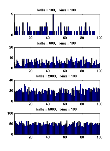}[/math] Figure 1 Due to the symmetry. All [math]\displaystyle{ X_i }[/math] have the same distribution. Apply the union bound again, [math]\displaystyle{ \begin{align} \Pr\left[\max_{1\le i\le n}X_i\ge M\right] &= \Pr\left[(X_1\ge M) \vee (X_2\ge M) \vee\cdots\vee (X_n\ge M)\right]\\ &\le n\Pr[X_1\ge M]\\ &\le n\left(\frac{e}{M}\right)^M. \end{align} }[/math] When [math]\displaystyle{ M=3\ln n/\ln\ln n }[/math], [math]\displaystyle{ \begin{align} \left(\frac{e}{M}\right)^M &= \left(\frac{e\ln\ln n}{3\ln n}\right)^{3\ln n/\ln\ln n}\\ &\lt \left(\frac{\ln\ln n}{\ln n}\right)^{3\ln n/\ln\ln n}\\ &= e^{3(\ln\ln\ln n-\ln\ln n)\ln n/\ln\ln n}\\ &= e^{-3\ln n+3\ln\ln\ln n\ln n/\ln\ln n}\\ &\le e^{-2\ln n}\\ &= \frac{1}{n^2}. \end{align} }[/math] Therefore, [math]\displaystyle{ \begin{align} \Pr\left[\max_{1\le i\le n}X_i\ge \frac{3\ln n}{\ln\ln n}\right] &\le n\left(\frac{e}{M}\right)^M &\lt \frac{1}{n}. \end{align} }[/math] [math]\displaystyle{ \square }[/math]

When [math]\displaystyle{ m\gt n }[/math], Figure 1 illustrates the results of several random experiments, which show that the distribution of the loads of bins becomes more even as the number of balls grows larger than the number of bins.

Formally, it can be proved that for [math]\displaystyle{ m=\Omega(n\log n) }[/math], with high probability, the maximum load is within [math]\displaystyle{ O\left(\frac{m}{n}\right) }[/math], which is asymptotically equal to the average load.

Universal Hashing

Hashing is one of the oldest tools in Computer Science. Knuth's memorandum in 1963 on analysis of hash tables is now considered to be the birth of the area of analysis of algorithms.

• Knuth. Notes on "open" addressing, July 22 1963. Unpublished memorandum.

The idea of hashing is simple: an unknown set [math]\displaystyle{ S }[/math] of [math]\displaystyle{ n }[/math] data items (or keys) are drawn from a large universe [math]\displaystyle{ U=[N] }[/math] where [math]\displaystyle{ N\gg n }[/math]; in order to store [math]\displaystyle{ S }[/math] in a table of [math]\displaystyle{ M }[/math] entries (slots), we assume a consistent mapping (called a hash function) from the universe [math]\displaystyle{ U }[/math] to a small range [math]\displaystyle{ [M] }[/math].

This idea seems clever: we use a consistent mapping to deal with an arbitrary unknown data set. However, there is a fundamental flaw for hashing.

• For sufficiently large universe ([math]\displaystyle{ N\gt M(n-1) }[/math]), for any function, there exists a bad data set [math]\displaystyle{ S }[/math], such that all items in [math]\displaystyle{ S }[/math] are mapped to the same entry in the table.

A simple use of pigeonhole principle can prove the above statement.

To overcome this situation, randomization is introduced into hashing. We assume that the hash function is a random mapping from [math]\displaystyle{ [N] }[/math] to [math]\displaystyle{ [M] }[/math]. In order to ease the analysis, the following ideal assumption is used:

Simple Uniform Hash Assumption (SUHA or UHA, a.k.a. the random oracle model):

A uniform random function [math]\displaystyle{ h:[N]\rightarrow[M] }[/math] is available and the computation of [math]\displaystyle{ h }[/math] is efficient.

Families of universal hash functions

The assumption of completely random function simplifies the analysis. However, in practice, truly uniform random hash function is extremely expensive to compute and store. Thus, this simple assumption can hardly represent the reality.

There are two approaches for implementing practical hash functions. One is to use ad hoc implementations and wish they may work. The other approach is to construct class of hash functions which are efficient to compute and store but with weaker randomness guarantees, and then analyze the applications of hash functions based on this weaker assumption of randomness.

This route was took by Carter and Wegman in 1977 while they introduced universal families of hash functions.

Definition (universal hash families)

Let [math]\displaystyle{ [N] }[/math] be a universe with [math]\displaystyle{ N\ge M }[/math]. A family of hash functions [math]\displaystyle{ \mathcal{H} }[/math] from [math]\displaystyle{ [N] }[/math] to [math]\displaystyle{ [M] }[/math] is said to be [math]\displaystyle{ k }[/math]-universal if, for any items [math]\displaystyle{ x_1,x_2,\ldots,x_k\in [N] }[/math] and for a hash function [math]\displaystyle{ h }[/math] chosen uniformly at random from [math]\displaystyle{ \mathcal{H} }[/math], we have [math]\displaystyle{ \Pr[h(x_1)=h(x_2)=\cdots=h(x_k)]\le\frac{1}{M^{k-1}}. }[/math] A family of hash functions [math]\displaystyle{ \mathcal{H} }[/math] from [math]\displaystyle{ [N] }[/math] to [math]\displaystyle{ [M] }[/math] is said to be strongly [math]\displaystyle{ k }[/math]-universal if, for any items [math]\displaystyle{ x_1,x_2,\ldots,x_k\in [N] }[/math], any values [math]\displaystyle{ y_1,y_2,\ldots,y_k\in[M] }[/math], and for a hash function [math]\displaystyle{ h }[/math] chosen uniformly at random from [math]\displaystyle{ \mathcal{H} }[/math], we have [math]\displaystyle{ \Pr[h(x_1)=y_1\wedge h(x_2)=y_2 \wedge \cdots \wedge h(x_k)=y_k]=\frac{1}{M^{k}}. }[/math]

In particular, for a 2-universal family [math]\displaystyle{ \mathcal{H} }[/math], for any elements [math]\displaystyle{ x_1,x_2\in[N] }[/math], a uniform random [math]\displaystyle{ h\in\mathcal{H} }[/math] has

[math]\displaystyle{ \Pr[h(x_1)=h(x_2)]\le\frac{1}{M}. }[/math]

For a strongly 2-universal family [math]\displaystyle{ \mathcal{H} }[/math], for any elements [math]\displaystyle{ x_1,x_2\in[N] }[/math] and any values [math]\displaystyle{ y_1,y_2\in[M] }[/math], a uniform random [math]\displaystyle{ h\in\mathcal{H} }[/math] has

[math]\displaystyle{ \Pr[h(x_1)=y_1\wedge h(x_2)=y_2]=\frac{1}{M^2}. }[/math]

This behavior is exactly the same as uniform random hash functions on any pair of inputs. For this reason, a strongly 2-universal hash family are also called pairwise independent hash functions.

2-universal hash families

The construction of pairwise independent random variables via modulo a prime introduced in Section 1 already provides a way of constructing a strongly 2-universal hash family.

Let [math]\displaystyle{ p }[/math] be a prime. The function [math]\displaystyle{ h_{a,b}:[p]\rightarrow [p] }[/math] is defined by

[math]\displaystyle{ h_{a,b}(x)=(ax+b)\bmod p, }[/math]

and the family is

[math]\displaystyle{ \mathcal{H}=\{h_{a,b}\mid a,b\in[p]\}. }[/math]

Lemma

[math]\displaystyle{ \mathcal{H} }[/math] is strongly 2-universal.

Proof. In Section 1, we have proved the pairwise independence of the sequence of [math]\displaystyle{ (a i+b)\bmod p }[/math], for [math]\displaystyle{ i=0,1,\ldots, p-1 }[/math], which directly implies that [math]\displaystyle{ \mathcal{H} }[/math] is strongly 2-universal. [math]\displaystyle{ \square }[/math]

The original construction of Carter-Wegman

What if we want to have hash functions from [math]\displaystyle{ [N] }[/math] to [math]\displaystyle{ [M] }[/math] for non-prime [math]\displaystyle{ N }[/math] and [math]\displaystyle{ M }[/math]? Carter and Wegman developed the following method.

Suppose that the universe is [math]\displaystyle{ [N] }[/math], and the functions map [math]\displaystyle{ [N] }[/math] to [math]\displaystyle{ [M] }[/math], where [math]\displaystyle{ N\ge M }[/math]. For some prime [math]\displaystyle{ p\ge N }[/math], let

[math]\displaystyle{ h_{a,b}(x)=((ax+b)\bmod p)\bmod M, }[/math]

and the family

[math]\displaystyle{ \mathcal{H}=\{h_{a,b}\mid 1\le a\le p-1, b\in[p]\}. }[/math]

Note that unlike the first construction, now [math]\displaystyle{ a\neq 0 }[/math].

Lemma (Carter-Wegman)

[math]\displaystyle{ \mathcal{H} }[/math] is 2-universal.

Proof. Due to the definition of [math]\displaystyle{ \mathcal{H} }[/math], there are [math]\displaystyle{ p(p-1) }[/math] many different hash functions in [math]\displaystyle{ \mathcal{H} }[/math], because each hash function in [math]\displaystyle{ \mathcal{H} }[/math] corresponds to a pair of [math]\displaystyle{ 1\le a\le p-1 }[/math] and [math]\displaystyle{ b\in[p] }[/math]. We only need to count for any particular pair of [math]\displaystyle{ x_1,x_2\in[N] }[/math] that [math]\displaystyle{ x_1\neq x_2 }[/math], the number of hash functions that [math]\displaystyle{ h(x_1)=h(x_2) }[/math]. We first note that for any [math]\displaystyle{ x_1\neq x_2 }[/math], [math]\displaystyle{ a x_1+b\not\equiv a x_2+b \pmod p }[/math]. This is because [math]\displaystyle{ a x_1+b\equiv a x_2+b \pmod p }[/math] would imply that [math]\displaystyle{ a(x_1-x_2)\equiv 0\pmod p }[/math], which can never happen since [math]\displaystyle{ 1\le a\le p-1 }[/math] and [math]\displaystyle{ x_1\neq x_2 }[/math] (note that [math]\displaystyle{ x_1,x_2\in[N] }[/math] for an [math]\displaystyle{ N\le p }[/math]). Therefore, we can assume that [math]\displaystyle{ (a x_1+b)\bmod p=u }[/math] and [math]\displaystyle{ (a x_2+b)\bmod p=v }[/math] for [math]\displaystyle{ u\neq v }[/math]. By linear algebra (over finite field), for any [math]\displaystyle{ x_1,x_2\in[N] }[/math] that [math]\displaystyle{ x_1\neq x_2 }[/math], for any [math]\displaystyle{ u,v\in[p] }[/math] that [math]\displaystyle{ u\neq v }[/math], there is exact one solution to [math]\displaystyle{ (a,b) }[/math] satisfying: [math]\displaystyle{ \begin{cases} a x_1+b \equiv u \pmod p\\ a x_2+b \equiv v \pmod p. \end{cases} }[/math] After modulo [math]\displaystyle{ M }[/math], every [math]\displaystyle{ u\in[p] }[/math] has at most [math]\displaystyle{ \lceil p/M\rceil -1 }[/math] many [math]\displaystyle{ v\in[p] }[/math] that [math]\displaystyle{ v\neq u }[/math] but [math]\displaystyle{ v\equiv u\pmod M }[/math]. Therefore, for every pair of [math]\displaystyle{ x_1,x_2\in[N] }[/math] that [math]\displaystyle{ x_1\neq x_2 }[/math], there exist at most [math]\displaystyle{ p(\lceil p/M\rceil -1)\le p(p-1)/M }[/math] pairs of [math]\displaystyle{ 1\le a\le p-1 }[/math] and [math]\displaystyle{ b\in[p] }[/math] such that [math]\displaystyle{ ((ax_1+b)\bmod p)\bmod M=((ax_2+b)\bmod p)\bmod M }[/math], which means there are at most [math]\displaystyle{ p(p-1)/M }[/math] many hash functions [math]\displaystyle{ h\in\mathcal{H} }[/math] having [math]\displaystyle{ h(x_1)=h(x_2) }[/math] for [math]\displaystyle{ x_1\neq x_2 }[/math]. For [math]\displaystyle{ h }[/math] uniformly chosen from [math]\displaystyle{ \mathcal{H} }[/math], for any [math]\displaystyle{ x_1\neq x_2 }[/math], [math]\displaystyle{ \Pr[h(x_1)=h(x_2)]\le \frac{p(p-1)/M}{p(p-1)}=\frac{1}{M}. }[/math] We prove that [math]\displaystyle{ \mathcal{H} }[/math] is 2-universal. [math]\displaystyle{ \square }[/math]

A construction used in practice

The main issue of Carter-Wegman construction is the efficiency. The mod operation is very slow, and has been so for more than 30 years.

The following construction is due to Dietzfelbinger et al. It was published in 1997 and has been practically used in various applications of universal hashing.

The family of hash functions is from [math]\displaystyle{ [2^u] }[/math] to [math]\displaystyle{ [2^v] }[/math]. With a binary representation, the functions map binary strings of length [math]\displaystyle{ u }[/math] to binary strings of length [math]\displaystyle{ v }[/math]. Let

[math]\displaystyle{ h_{a}(x)=\left\lfloor\frac{a\cdot x\bmod 2^u}{2^{u-v}}\right\rfloor, }[/math]

and the family

[math]\displaystyle{ \mathcal{H}=\{h_{a}\mid a\in[2^v]\mbox{ and }a\mbox{ is odd}\}. }[/math]

This family of hash functions does not exactly meet the requirement of 2-universal family. However, Dietzfelbinger et al proved that [math]\displaystyle{ \mathcal{H} }[/math] is close to a 2-universal family. Specifically, for any input values [math]\displaystyle{ x_1,x_2\in[2^u] }[/math], for a uniformly random [math]\displaystyle{ h\in\mathcal{H} }[/math],

[math]\displaystyle{ \Pr[h(x_1)=h(x_2)]\le\frac{1}{2^{v-1}}. }[/math]

So [math]\displaystyle{ \mathcal{H} }[/math] is within an approximation ratio of 2 to being 2-universal. The proof uses the fact that odd numbers are relative prime to a power of 2.

The function is extremely simple to compute in c language. We exploit that C-multiplication (*) of unsigned u-bit numbers is done [math]\displaystyle{ \bmod 2^u }[/math], and have a one-line C-code for computing the hash function:

h_a(x) = (a*x)>>(u-v)

The bit-wise shifting is a lot faster than modular. It explains the popularity of this scheme in practice than the original Carter-Wegman construction.

Collision number

Consider a 2-universal family [math]\displaystyle{ \mathcal{H} }[/math] of hash functions from [math]\displaystyle{ [N] }[/math] to [math]\displaystyle{ [M] }[/math]. Let [math]\displaystyle{ h }[/math] be a hash function chosen uniformly from [math]\displaystyle{ \mathcal{H} }[/math]. For a fixed set [math]\displaystyle{ S }[/math] of [math]\displaystyle{ n }[/math] distinct elements from [math]\displaystyle{ [N] }[/math], say [math]\displaystyle{ S=\{x_1,x_2,\ldots,x_n\} }[/math], the elements are mapped to the hash values [math]\displaystyle{ h(x_1), h(x_2), \ldots, h(x_n) }[/math]. This can be seen as throwing [math]\displaystyle{ n }[/math] balls to [math]\displaystyle{ M }[/math] bins, with pairwise independent choices of bins.

As in the balls-into-bins with full independence, we are curious about the questions such as the birthday problem or the maximum load. These questions are interesting not only because they are natural to ask in a balls-into-bins setting, but in the context of hashing, they are closely related to the performance of hash functions.

The old techniques for analyzing balls-into-bins rely too much on the independence of the choice of the bin for each ball, therefore can hardly be extended to the setting of 2-universal hash families. However, it turns out several balls-into-bins questions can somehow be answered by analyzing a very natural quantity: the number of collision pairs.

A collision pair for hashing is a pair of elements [math]\displaystyle{ x_1,x_2\in S }[/math] which are mapped to the same hash value, i.e. [math]\displaystyle{ h(x_1)=h(x_2) }[/math]. Formally, for a fixed set of elements [math]\displaystyle{ S=\{x_1,x_2,\ldots,x_n\} }[/math], for any [math]\displaystyle{ 1\le i,j\le n }[/math], let the random variable

[math]\displaystyle{ X_{ij} = \begin{cases} 1 & \text{if }h(x_i)=h(x_j),\\ 0 & \text{otherwise.} \end{cases} }[/math]

The total number of collision pairs among the [math]\displaystyle{ n }[/math] items [math]\displaystyle{ x_1,x_2,\ldots,x_n }[/math] is

[math]\displaystyle{ X=\sum_{i\lt j} X_{ij}.\, }[/math]

Since [math]\displaystyle{ \mathcal{H} }[/math] is 2-universal, for any [math]\displaystyle{ i\neq j }[/math],

[math]\displaystyle{ \Pr[X_{ij}=1]=\Pr[h(x_i)=h(x_j)]\le\frac{1}{M}. }[/math]

The expected number of collision pairs is

[math]\displaystyle{ \mathbf{E}[X]=\mathbf{E}\left[\sum_{i\lt j}X_{ij}\right]=\sum_{i\lt j}\mathbf{E}[X_{ij}]=\sum_{i\lt j}\Pr[X_{ij}=1]\le{n\choose 2}\frac{1}{M}\lt \frac{n^2}{2M}. }[/math]

In particular, for [math]\displaystyle{ n=M }[/math], i.e. [math]\displaystyle{ n }[/math] items are mapped to [math]\displaystyle{ n }[/math] hash values by a pairwise independent hash function, the expected collision number is [math]\displaystyle{ \mathbf{E}[X]\lt \frac{n^2}{2M}=\frac{n}{2} }[/math].

Birthday problem

In the context of hash functions, the birthday problem ask for the probability that there is no collision at all. Since collision is something that we want to avoid in the applications of hash functions, we would like to lower bound the probability of zero-collision, i.e. to upper bound the probability that there exists a collision pair.

The above analysis gives us an estimation on the expected number of collision pairs, such that [math]\displaystyle{ \mathbf{E}[X]\lt \frac{n^2}{2M} }[/math]. Apply the Markov's inequality, for [math]\displaystyle{ 0\lt \epsilon\lt 1 }[/math], we have

[math]\displaystyle{ \Pr\left[X\ge \frac{n^2}{2\epsilon M}\right]\le\Pr\left[X\ge \frac{1}{\epsilon}\mathbf{E}[X]\right]\le\epsilon. }[/math]

When [math]\displaystyle{ n\le\sqrt{2\epsilon M} }[/math], the number of collision pairs is [math]\displaystyle{ X\ge1 }[/math] with probability at most [math]\displaystyle{ \epsilon }[/math], therefore with probability at least [math]\displaystyle{ 1-\epsilon }[/math], there is no collision at all. Therefore, we have the following theorem.

Theorem

If [math]\displaystyle{ h }[/math] is chosen uniformly from a 2-universal family of hash functions mapping the universe [math]\displaystyle{ [N] }[/math] to [math]\displaystyle{ [M] }[/math] where [math]\displaystyle{ N\ge M }[/math], then for any set [math]\displaystyle{ S\subset [N] }[/math] of [math]\displaystyle{ n }[/math] items, where [math]\displaystyle{ n\le\sqrt{2\epsilon M} }[/math], the probability that there exits a collision pair is [math]\displaystyle{ \Pr[\mbox{collision occurs}]\le\epsilon. }[/math]

Recall that for mutually independent choices of bins, for some [math]\displaystyle{ n=\sqrt{2M\ln(1/\epsilon)} }[/math], the probability that a collision occurs is about [math]\displaystyle{ \epsilon }[/math]. For constant [math]\displaystyle{ \epsilon }[/math], this gives an essentially same bound as the pairwise independent setting. Therefore, the behavior of pairwise independent hash function is essentially the same as the uniform random hash function for the birthday problem. This is easy to understand, because birthday problem is about the behavior of collisions, and the definition of 2-universal hash function can be interpreted as "functions that the probability of collision is as low as a uniform random function".

Perfect Hashing

Perfect hashing is a data structure for storing a static dictionary. In a static dictionary, a set [math]\displaystyle{ S }[/math] of [math]\displaystyle{ n }[/math] items from the universe [math]\displaystyle{ [N] }[/math] are preprocessed and stored in a table. Once the table is constructed, it will nit be changed any more, but will only be used for search operations: a search for an item gives the location of the item in the table or returns that the item is not in the table. You may think of an application that we store an encyclopedia in a DVD, so that searches are very efficient but there will be no updates to the data.

This problem can be solved by binary search on a sorted table or balanced search trees in [math]\displaystyle{ O(\log n) }[/math] time for a set [math]\displaystyle{ S }[/math] of [math]\displaystyle{ n }[/math] elements. We show how to solve this problem with [math]\displaystyle{ O(1) }[/math] time by perfect hashing.

Perfect hashing using quadratic space

The idea of perfect hashing is that we use a hash function [math]\displaystyle{ h }[/math] to map the [math]\displaystyle{ n }[/math] items to distinct entries of the table; store every item [math]\displaystyle{ x\in S }[/math] in the entry [math]\displaystyle{ h(x) }[/math]; and also store the hash function [math]\displaystyle{ h }[/math] in a fixed location in the table (usually the beginning of the table). The algorithm for searching for an item is as follows:

search for [math]\displaystyle{ x }[/math] in table [math]\displaystyle{ T }[/math]:

1. retrieve [math]\displaystyle{ h }[/math] from a fixed location in the table;
2. if [math]\displaystyle{ x=T[h(x)] }[/math] return [math]\displaystyle{ h(x) }[/math]; else return NOT_FOUND;

This scheme works as long as that the hash function satisfies the following two conditions:

• The description of [math]\displaystyle{ h }[/math] is sufficiently short, so that [math]\displaystyle{ h }[/math] can be stored in one entry (or in constant many entries) of the table.
• [math]\displaystyle{ h }[/math] has no collisions on [math]\displaystyle{ S }[/math], i.e. there is no pair of items [math]\displaystyle{ x_1,x_2\in S }[/math] that are mapped to the same value by [math]\displaystyle{ h }[/math].

The first condition is easy to guarantee for 2-universal hash families. As shown by Carter-Wegman construction, a 2-universal hash function can be uniquely represented by two integers [math]\displaystyle{ a }[/math] and [math]\displaystyle{ b }[/math], which can be stored in two entries (or just one, if the word length is sufficiently large) of the table.

Our discussion is now focused on the second condition. We find that it relies on the perfectness of the hash function for a data set [math]\displaystyle{ S }[/math].

A hash function [math]\displaystyle{ h }[/math] is perfect for a set [math]\displaystyle{ S }[/math] of items if [math]\displaystyle{ h }[/math] maps all items in [math]\displaystyle{ S }[/math] to different values, i.e. there is no collision.

We have shown by the birthday problem for 2-universal hashing that when [math]\displaystyle{ n }[/math] items are mapped to [math]\displaystyle{ n^2 }[/math] values, for an [math]\displaystyle{ h }[/math] chosen uniformly from a 2-universal family of hash functions, the probability that a collision occurs is at most 1/2. Thus

[math]\displaystyle{ \Pr[h\mbox{ is perfect for }S]\ge\frac{1}{2} }[/math]

for a table of [math]\displaystyle{ n^2 }[/math] entries.

The construction of perfect hashing is straightforward then:

For a set [math]\displaystyle{ S }[/math] of [math]\displaystyle{ n }[/math] elements:

1. uniformly choose an [math]\displaystyle{ h }[/math] from a 2-universal family [math]\displaystyle{ \mathcal{H} }[/math]; (for Carter-Wegman's construction, it means uniformly choose two integer [math]\displaystyle{ 1\le a\le p-1 }[/math] and [math]\displaystyle{ b\in[p] }[/math] for a sufficiently large prime [math]\displaystyle{ p }[/math].)
2. check whether [math]\displaystyle{ h }[/math] is perfect for [math]\displaystyle{ S }[/math];
3. if [math]\displaystyle{ h }[/math] is NOT perfect for [math]\displaystyle{ S }[/math], start over again; otherwise, construct the table;

This is a Las Vegas randomized algorithm, which construct a perfect hashing for a fixed set [math]\displaystyle{ S }[/math] with expectedly at most two trials (due to geometric distribution). The resulting data structure is a [math]\displaystyle{ O(n^2) }[/math]-size static dictionary of [math]\displaystyle{ n }[/math] elements which answers every search in deterministic [math]\displaystyle{ O(1) }[/math] time.

FKS perfect hashing

In the last section we see how to use [math]\displaystyle{ O(n^2) }[/math] space and constant time for answering search in a set. Now we see how to do it with linear space and constant time. This solves the problem of searching asymptotically optimal for both time and space.

This was once seemingly impossible, until Yao's seminal paper:

• Yao. Should tables be sorted? Journal of the ACM (JACM), 1981.

Yao's paper shows a possibility of achieving linear space and constant time at the same time by exploiting the power of hashing, but assumes an unrealistically large universe.

Inspired by Yao's work, Fredman, Komlós, and Szemerédi discover the first linear-space and constant-time static dictionary in a realistic setting:

• Fredman, Komlós, and Szemerédi. Storing a sparse table with O(1) worst case access time. Journal of the ACM (JACM), 1984.

The idea of FKS hashing is to arrange hash table in two levels:

• In the first level, [math]\displaystyle{ n }[/math] items are hashed to [math]\displaystyle{ n }[/math] buckets by a 2-universal hash function [math]\displaystyle{ h }[/math].

Let [math]\displaystyle{ B_i }[/math] be the set of items hashed to the [math]\displaystyle{ i }[/math]th bucket.

• In the second level, construct a [math]\displaystyle{ |B_i|^2 }[/math]-size perfect hashing for each bucket [math]\displaystyle{ B_i }[/math].

The data structure can be stored in a table. The first few entries are reserved to store the primary hash function [math]\displaystyle{ h }[/math]. To help the searching algorithm locate a bucket, we use the next [math]\displaystyle{ n }[/math] entries of the table as the "pointers" to the bucket: each entry stores the address of the first entry of the space to store a bucket. In the rest of table, the [math]\displaystyle{ n }[/math] buckets are stored in order, each using a [math]\displaystyle{ |B_i|^2 }[/math] space as required by perfect hashing.

It is easy to see that the search time is constant. To search for an item [math]\displaystyle{ x }[/math], the algorithm does the followings:

• Retrieve [math]\displaystyle{ h }[/math].
• Retrieve the address for bucket [math]\displaystyle{ h(x) }[/math].
• Search by perfect hashing within bucket [math]\displaystyle{ h(x) }[/math].

Each line takes constant time. So the worst-case search time is constant.

We then need to guarantee that the space is linear to [math]\displaystyle{ n }[/math]. At the first glance, this seems impossible because each instance of perfect hashing for a bucket costs a square-size of space. We will prove that although the individual buckets use square-sized spaces, the sum of the them is still linear.

For a fixed set [math]\displaystyle{ S }[/math] of [math]\displaystyle{ n }[/math] items, for a hash function [math]\displaystyle{ h }[/math] chosen uniformly from a 2-universe family which maps the items to [math]\displaystyle{ [n] }[/math], called [math]\displaystyle{ n }[/math] buckets, let [math]\displaystyle{ Y_i=|B_i| }[/math] be the number of items in [math]\displaystyle{ S }[/math] mapped to the [math]\displaystyle{ i }[/math]th bucket. We are going to bound the following quantity:

[math]\displaystyle{ Y=\sum_{i=1}^n Y_i^2. }[/math]

Since each bucket [math]\displaystyle{ B_i }[/math] use a space of [math]\displaystyle{ Y_i^2 }[/math] for perfect hashing. [math]\displaystyle{ Y }[/math] gives the size of the space for storing the buckets.

We will show that [math]\displaystyle{ Y }[/math] is related to the total number of collision pairs. (Indeed, the number of collision pairs can be computed by a degree-2 polynomial, just like [math]\displaystyle{ Y }[/math].)

Note that a bucket of [math]\displaystyle{ Y_i }[/math] items contributes [math]\displaystyle{ {Y_i\choose 2} }[/math] collision pairs. Let [math]\displaystyle{ X }[/math] be the total number of collision pairs. [math]\displaystyle{ X }[/math] can be computed by summing over the collision pairs in every bucket:

[math]\displaystyle{ X=\sum_{i=1}^n{Y_i\choose 2}=\sum_{i=1}^n\frac{Y_i(Y_i-1)}{2}=\frac{1}{2}\left(\sum_{i=1}^nY_i^2-\sum_{i=1}^nY_i\right)=\frac{1}{2}\left(\sum_{i=1}^nY_i^2-n\right). }[/math]

Therefore, the sum of squares of the sizes of buckets is related to collision number by:

[math]\displaystyle{ \sum_{i=1}^nY_i^2=2X+n. }[/math]

By our analysis of the collision number, we know that for [math]\displaystyle{ n }[/math] items mapped to [math]\displaystyle{ n }[/math] buckets, the expected number of collision pairs is: [math]\displaystyle{ \mathbf{E}[X]\le \frac{n}{2} }[/math]. Thus,

[math]\displaystyle{ \mathbf{E}\left[\sum_{i=1}^nY_i^2\right]=\mathbf{E}[2X+n]\le 2n. }[/math]

Due to Markov's inequality, [math]\displaystyle{ \sum_{i=1}^nY_i^2=O(n) }[/math] with a constant probability. For any set [math]\displaystyle{ S }[/math], we can find a suitable [math]\displaystyle{ h }[/math] after expected constant number of trials, and FKS can be constructed with guaranteed (instead of expected) linear-size which answers each search in constant time.